2 Quick start
In this chapter, we illustrate the main steps of the epiregulon workflow.
2.1 Prepare data
We need the following components to perform GRN analysis:
1. Peak matrix from scATAC-seq
2. Paired gene expression matrix from scRNA-seq
3. Dimensionality reduction matrix
We download an example PBMC dataset from the scMultiome package.
# load the MAE object
library(scMultiome)
library(epiregulon)

# Download the example dataset
mae <- scMultiome::PBMC_10x()

# Load peak matrix
PeakMatrix <- mae[["PeakMatrix"]]

# Load expression matrix
GeneExpressionMatrix <- mae[["GeneExpressionMatrix"]]
Visualize singleCellExperiment by UMAP
scater::plotReducedDim(GeneExpressionMatrix,
                       dimred = "UMAP_RNA",
                       text_by = "cell_type",
                       colour_by = "cell_type",
                       point_size = 0.3,
                       point_alpha = 0.3)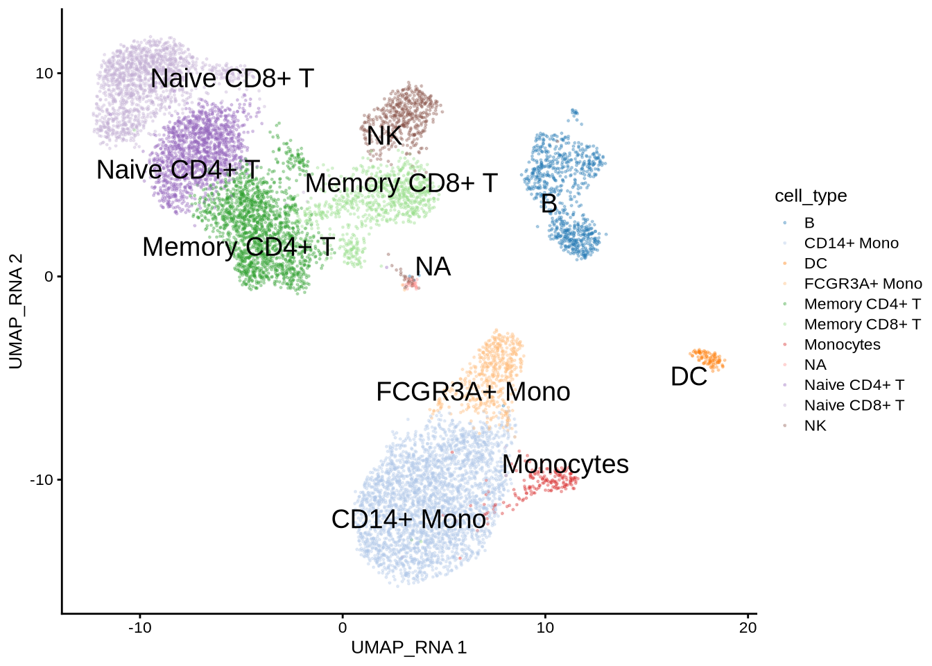
2.2 Retrieve bulk TF ChIP-seq binding sites
We retrieve a GRangesList object containing the binding sites of transcription factors and co-regulators. These binding sites are derived from bulk ChIP-seq data in the ChIP-Atlas and ENCODE databases. For further information on how these peaks are derived, please refer to ?epiregulon::getTFMotifInfo. Currently, only human genomes hg19 and hg38 and mouse mm10 are supported.
## GRangesList object of length 1377:
## $AEBP2
## GRanges object with 2700 ranges and 0 metadata columns:
##          seqnames            ranges strand
##             <Rle>         <IRanges>  <Rle>
##      [1]     chr1        9792-10446      *
##      [2]     chr1     942105-942400      *
##      [3]     chr1     984486-984781      *
##      [4]     chr1   3068932-3069282      *
##      [5]     chr1   3069411-3069950      *
##      ...      ...               ...    ...
##   [2696]     chrY   8465261-8465730      *
##   [2697]     chrY 11721744-11722260      *
##   [2698]     chrY 11747448-11747964      *
##   [2699]     chrY 19302661-19303134      *
##   [2700]     chrY 19985662-19985982      *
##   -------
##   seqinfo: 25 sequences from an unspecified genome; no seqlengths
##
## ...
## <1376 more elements>
2.3 Link ATAC-seq peaks to target genes
Next, we link ATAC-seq peaks to their putative target genes. We assign a peak to genes within a size window (default ±250kb) if the chromatin accessibility of the peak and expression of the target genes are highly correlated. To compute correlation, we first create cell aggregates by performing k-means clustering on the reduced dimensionality matrix. To estimate the optimal number of cells per cluster we run optimizeMetacellNumber.
set.seed(1010)
cellNum <- optimizeMetacellNumber(expMatrix = GeneExpressionMatrix,
                                  peakMatrix = PeakMatrix,
                                  exp_assay = "normalizedCounts",
                                  peak_assay = "counts",
                                  reducedDim = reducedDim(GeneExpressionMatrix, "LSI_RNA"),
                                  BPPARAM = BiocParallel::SerialParam(progressbar = FALSE))
cellNum object is then provided as an argument to calculateP2G.
set.seed(1010)
p2g <- calculateP2G(peakMatrix = PeakMatrix,
                    expMatrix = GeneExpressionMatrix,
                    reducedDim = reducedDim(GeneExpressionMatrix, "LSI_RNA"),
                    exp_assay = "normalizedCounts",
                    peak_assay = "counts")
## Using epiregulon to compute peak to gene links...## Creating metacells...
## Looking for regulatory elements near target genes...
## Computing correlations...
## | | | 0% | |=== | 2% | |===== | 5% | |======== | 7% | |=========== | 9% | |============== | 11% | |================ | 14% | |=================== | 16% | |====================== | 18% | |========================= | 20% | |=========================== | 23% | |============================== | 25% | |================================= | 27% | |=================================== | 30% | |====================================== | 32% | |========================================= | 34% | |============================================ | 36% | |============================================== | 39% | |================================================= | 41% | |==================================================== | 43% | |======================================================= | 45% | |========================================================= | 48% | |============================================================ | 50% | |=============================================================== | 52% | |================================================================= | 55% | |==================================================================== | 57% | |======================================================================= | 59% | |========================================================================== | 61% | |============================================================================ | 64% | |=============================================================================== | 66% | |================================================================================== | 68% | |===================================================================================== | 70% | |======================================================================================= | 73% | |========================================================================================== | 75% | |============================================================================================= | 77% | |=============================================================================================== | 80% | |================================================================================================== | 82% | |===================================================================================================== | 84% | |======================================================================================================== | 86% | |========================================================================================================== | 89% | |============================================================================================================= | 91% | |================================================================================================================ | 93% | |=================================================================================================================== | 95% | |===================================================================================================================== | 98% | |========================================================================================================================| 100%
##
## | | | 0% | |======================== | 20% | |================================================ | 40% | |======================================================================== | 60% | |================================================================================================ | 80% | |========================================================================================================================| 100%## DataFrame with 67644 rows and 10 columns
## idxATAC chr start end idxRNA target Correlation p_val_peak_gene FDR_peak_gene distance
## <integer> <character> <integer> <integer> <integer> <array> <matrix> <matrix> <matrix> <integer>
## 1 1 chr1 817086 817586 17 LINC00115 0.487936 0.0397870 0.616636 9934
## 2 10 chr1 897218 897718 30 HES4 0.464881 0.0456846 0.625393 102261
## 3 27 chr1 955434 955934 30 HES4 0.552958 0.0248449 0.566187 44045
## 4 27 chr1 955434 955934 33 AGRN 0.498275 0.0366621 0.603988 64184
## 5 29 chr1 959712 960212 31 ISG15 -0.398968 0.0247077 0.566187 40924
## ... ... ... ... ... ... ... ... ... ... ...
## 67640 159255 chrX 154799001 154799501 36414 DKC1 -0.378386 0.0295832 0.578736 36259
## 67641 159255 chrX 154799001 154799501 36415 MPP1 0.644579 0.0118173 0.506844 5894
## 67642 159255 chrX 154799001 154799501 36419 F8A1 -0.395646 0.0252025 0.566187 86846
## 67643 159256 chrX 154800772 154801272 36415 MPP1 0.610599 0.0158884 0.532984 4123
## 67644 159256 chrX 154800772 154801272 36419 F8A1 -0.393617 0.0257158 0.568362 850752.4 Add TF motif binding to peaks
We next add the TF binding information by overlapping ATAC peaks with ChIP-seq peaks. The output is a data frame object with three columns:
idxATAC- index in the peak matrixidxTF- index in the gene expression matrix corresponding to the transcription factortf- name of the transcription factor
##   idxATAC idxTF    tf
## 1       1    16  ATF1
## 2       1    17  ATF2
## 3       1    18  ATF3
## 4       1    21  ATF7
## 5       1    35 BRCA2
## 6       1    36  BRD4
2.5 Generate regulons
We then generate a DataFrame object representing the inferred regulons, indicating target genes, transcription factors, and regulatory elements.
## DataFrame with 8418612 rows and 12 columns
##           idxATAC         chr     start       end    idxRNA    target      corr p_val_peak_gene FDR_peak_gene  distance     idxTF
##         <integer> <character> <integer> <integer> <integer>   <array>  <matrix>        <matrix>      <matrix> <integer> <integer>
## 1               1        chr1    817086    817586        17 LINC00115  0.487936        0.039787      0.616636      9934        16
## 2               1        chr1    817086    817586        17 LINC00115  0.487936        0.039787      0.616636      9934        17
## 3               1        chr1    817086    817586        17 LINC00115  0.487936        0.039787      0.616636      9934        18
## 4               1        chr1    817086    817586        17 LINC00115  0.487936        0.039787      0.616636      9934        21
## 5               1        chr1    817086    817586        17 LINC00115  0.487936        0.039787      0.616636      9934        35
## ...           ...         ...       ...       ...       ...       ...       ...             ...           ...       ...       ...
## 8418608    159256        chrX 154800772 154801272     36419      F8A1 -0.393617       0.0257158      0.568362     85075       979
## 8418609    159256        chrX 154800772 154801272     36419      F8A1 -0.393617       0.0257158      0.568362     85075       991
## 8418610    159256        chrX 154800772 154801272     36419      F8A1 -0.393617       0.0257158      0.568362     85075      1018
## 8418611    159256        chrX 154800772 154801272     36419      F8A1 -0.393617       0.0257158      0.568362     85075      1020
## 8418612    159256        chrX 154800772 154801272     36419      F8A1 -0.393617       0.0257158      0.568362     85075      1335
##                      tf
##             <character>
## 1                  ATF1
## 2                  ATF2
## 3                  ATF3
## 4                  ATF7
## 5                 BRCA2
## ...                 ...
## 8418608             MNT
## 8418609            NFIA
## 8418610          POLR2A
## 8418611 POLR2AphosphoS5
## 8418612          ZNF766
2.6 Prune network (recommended)
Since our regulons could contain false connections, we apply the pruning function.
pruned.regulon <- pruneRegulon(expMatrix = GeneExpressionMatrix,
                               exp_assay = "normalizedCounts",
                               peakMatrix = PeakMatrix,
                               peak_assay = "counts",
                               test = "chi.sq",
                               regulon,
                               prune_value = "pval",
                               regulon_cutoff = 0.05
                               )

pruned.regulon
## DataFrame with 2754396 rows and 15 columns
## idxATAC chr start end idxRNA target corr p_val_peak_gene FDR_peak_gene distance idxTF
## <integer> <character> <integer> <integer> <integer> <array> <matrix> <matrix> <matrix> <integer> <integer>
## 1 135 chr1 1207949 1208449 44 TNFRSF4 0.618308 0.01483209 0.528124 5702 887
## 2 135 chr1 1207949 1208449 43 TNFRSF18 0.686583 0.00836231 0.498760 2269 887
## 3 266 chr1 1686177 1686677 86 NADK 0.682560 0.00867039 0.499675 91791 887
## 4 991 chr1 8947075 8947575 222 CA6 0.581208 0.02000352 0.551146 1207 887
## 5 1103 chr1 9628994 9629494 233 SLC25A33 -0.545647 0.00456395 0.463887 89529 887
## ... ... ... ... ... ... ... ... ... ... ... ...
## 2754392 155544 chr22 50524937 50525437 23714 TYMP -0.378229 0.0296565 0.579085 4557 1377
## 2754393 155577 chr22 50582163 50582663 23714 TYMP -0.365791 0.0335423 0.595442 52167 1377
## 2754394 155577 chr22 50582163 50582663 23715 ODF3B -0.337503 0.0436050 0.623854 50086 1377
## 2754395 158053 chrX 106611664 106612164 36005 RADX 0.551794 0.0249989 0.566187 0 1377
## 2754396 158949 chrX 150547614 150548114 36307 MTM1 0.579942 0.0201796 0.551336 20503 1377
## tf pval stats qval
## <character> <matrix> <matrix> <matrix>
## 1 ADNP 3.83812e-09 34.70415 0.0286741
## 2 ADNP 1.15983e-04 14.85689 1.0000000
## 3 ADNP 2.14101e-07 26.90142 1.0000000
## 4 ADNP 2.09927e-03 9.46065 1.0000000
## 5 ADNP 1.01188e-03 10.80569 1.0000000
## ... ... ... ... ...
## 2754392 ZXDC 1.93434e-02 5.47020 1
## 2754393 ZXDC 4.48926e-04 12.31669 1
## 2754394 ZXDC 6.00511e-03 7.54877 1
## 2754395 ZXDC 3.72567e-06 21.40105 1
## 2754396 ZXDC 3.33531e-03 8.61432 12.7 Annotate regulon
Regulons can be annotated for further refinement. One such metric is the log fold change of gene expression in specified groups. Before running addLogFC function, we need to log-transform gene expression counts. In this example, we are interested in target genes differentially expressed in Naive CD4+ T cells.
# add 'logcounts' assay
GeneExpressionMatrix <- scuttle::logNormCounts(GeneExpressionMatrix)

regulon.FC <- addLogFC(expMatrix = GeneExpressionMatrix,
                       clusters = GeneExpressionMatrix$cell_type,
                       regulon = pruned.regulon,
                       pval.type = "any",
                       sig_type = "FDR",
                       assay.type = "logcounts",
                       logFC_condition=c('Naive CD4+ T')
)

regulon.FC
## DataFrame with 2754396 rows and 17 columns
## idxATAC chr start end idxRNA target corr p_val_peak_gene FDR_peak_gene distance idxTF
## <integer> <character> <integer> <integer> <integer> <array> <matrix> <matrix> <matrix> <integer> <integer>
## 1 135 chr1 1207949 1208449 44 TNFRSF4 0.618308 0.01483209 0.528124 5702 887
## 2 135 chr1 1207949 1208449 43 TNFRSF18 0.686583 0.00836231 0.498760 2269 887
## 3 266 chr1 1686177 1686677 86 NADK 0.682560 0.00867039 0.499675 91791 887
## 4 991 chr1 8947075 8947575 222 CA6 0.581208 0.02000352 0.551146 1207 887
## 5 1103 chr1 9628994 9629494 233 SLC25A33 -0.545647 0.00456395 0.463887 89529 887
## ... ... ... ... ... ... ... ... ... ... ... ...
## 2754392 155544 chr22 50524937 50525437 23714 TYMP -0.378229 0.0296565 0.579085 4557 1377
## 2754393 155577 chr22 50582163 50582663 23714 TYMP -0.365791 0.0335423 0.595442 52167 1377
## 2754394 155577 chr22 50582163 50582663 23715 ODF3B -0.337503 0.0436050 0.623854 50086 1377
## 2754395 158053 chrX 106611664 106612164 36005 RADX 0.551794 0.0249989 0.566187 0 1377
## 2754396 158949 chrX 150547614 150548114 36307 MTM1 0.579942 0.0201796 0.551336 20503 1377
## tf pval stats qval Naive CD4+ T.vs.rest.FDR Naive CD4+ T.vs.rest.logFC
## <character> <matrix> <matrix> <matrix> <numeric> <numeric>
## 1 ADNP 3.83812e-09 34.70415 0.0286741 1.24716e-40 -0.158980
## 2 ADNP 1.15983e-04 14.85689 1.0000000 2.07408e-28 -0.106426
## 3 ADNP 2.14101e-07 26.90142 1.0000000 4.93457e-177 -0.402145
## 4 ADNP 2.09927e-03 9.46065 1.0000000 1.74410e-35 -0.265716
## 5 ADNP 1.01188e-03 10.80569 1.0000000 5.97271e-65 -0.230591
## ... ... ... ... ... ... ...
## 2754392 ZXDC 1.93434e-02 5.47020 1 0.00000e+00 -2.3462477
## 2754393 ZXDC 4.48926e-04 12.31669 1 0.00000e+00 -2.3462477
## 2754394 ZXDC 6.00511e-03 7.54877 1 9.44166e-179 -0.3415591
## 2754395 ZXDC 3.72567e-06 21.40105 1 3.21089e-07 0.0323369
## 2754396 ZXDC 3.33531e-03 8.61432 1 2.88666e-23 0.1631049We can also annotate regulons for the presence of motifs at each regulatory element.
regulon.motif <- addMotifScore(regulon = pruned.regulon,
                                peaks = rowRanges(PeakMatrix),
                                species = "human",
                                genome = "hg38")
regulon.motif
## DataFrame with 2754396 rows and 16 columns
## idxATAC chr start end idxRNA target corr p_val_peak_gene FDR_peak_gene distance idxTF
## <integer> <character> <integer> <integer> <integer> <array> <matrix> <matrix> <matrix> <integer> <integer>
## 1 135 chr1 1207949 1208449 44 TNFRSF4 0.618308 0.01483209 0.528124 5702 887
## 2 135 chr1 1207949 1208449 43 TNFRSF18 0.686583 0.00836231 0.498760 2269 887
## 3 266 chr1 1686177 1686677 86 NADK 0.682560 0.00867039 0.499675 91791 887
## 4 991 chr1 8947075 8947575 222 CA6 0.581208 0.02000352 0.551146 1207 887
## 5 1103 chr1 9628994 9629494 233 SLC25A33 -0.545647 0.00456395 0.463887 89529 887
## ... ... ... ... ... ... ... ... ... ... ... ...
## 2754392 155544 chr22 50524937 50525437 23714 TYMP -0.378229 0.0296565 0.579085 4557 1377
## 2754393 155577 chr22 50582163 50582663 23714 TYMP -0.365791 0.0335423 0.595442 52167 1377
## 2754394 155577 chr22 50582163 50582663 23715 ODF3B -0.337503 0.0436050 0.623854 50086 1377
## 2754395 158053 chrX 106611664 106612164 36005 RADX 0.551794 0.0249989 0.566187 0 1377
## 2754396 158949 chrX 150547614 150548114 36307 MTM1 0.579942 0.0201796 0.551336 20503 1377
## tf pval stats qval motif
## <character> <matrix> <matrix> <matrix> <numeric>
## 1 ADNP 3.83812e-09 34.70415 0.0286741 NA
## 2 ADNP 1.15983e-04 14.85689 1.0000000 NA
## 3 ADNP 2.14101e-07 26.90142 1.0000000 NA
## 4 ADNP 2.09927e-03 9.46065 1.0000000 NA
## 5 ADNP 1.01188e-03 10.80569 1.0000000 NA
## ... ... ... ... ... ...
## 2754392 ZXDC 1.93434e-02 5.47020 1 NA
## 2754393 ZXDC 4.48926e-04 12.31669 1 NA
## 2754394 ZXDC 6.00511e-03 7.54877 1 NA
## 2754395 ZXDC 3.72567e-06 21.40105 1 NA
## 2754396 ZXDC 3.33531e-03 8.61432 1 NA2.8 Calculate TF activity
Finally, activities for a specific TF in each cell are computed by averaging expressions of target genes weighted by the test statistics of choice.
\[y=\frac{1}{n}\sum_{i=1}^{n} x_i * weights_i\]
where \(y\) is the activity of a TF for a cell,
\(n\) is the total number of targets for a TF,
\(x_i\) is the log count expression of target \(i\) where \(i\) in {1,2,…,n} and
\(weights_i\) is the weight of TF - target \(i\), calculated by running addWeights function.
regulon.w <- addWeights(regulon = pruned.regulon,
                        expMatrix  = GeneExpressionMatrix,
                        exp_assay  = "normalizedCounts",
                        peakMatrix = PeakMatrix,
                        peak_assay = "counts")


score.combine <- calculateActivity(expMatrix = GeneExpressionMatrix,
                                   regulon = regulon.w,
                                   mode = "weight",
                                   exp_assay = "normalizedCounts",
                                   normalize = FALSE)

score.combine[1:5,1:5]
## 5 x 5 sparse Matrix of class "dgCMatrix"
## PBMC_10k#GGTTGCATCCTGGCTT-1 PBMC_10k#GGTTGCGGTAAACAAG-1 PBMC_10k#TGTTCCTCATAAGTTC-1 PBMC_10k#CGACTAAGTAACGGGA-1
## ADNP 0.11379320 0.09052355 0.11310774 0.07767001
## AEBP2 0.03488950 0.06604866 0.06581493 0.07258739
## AFF1 0.09373167 0.08967789 0.10807508 0.06184494
## AFF4 0.11164763 0.10782789 0.13602988 0.07292949
## AGO1 0.09017644 0.07779564 0.08892206 0.05903171
## PBMC_10k#CTGCTCCCAAGGTCCT-1
## ADNP 0.1201884
## AEBP2 0.0780261
## AFF1 0.1136837
## AFF4 0.1392258
## AGO1 0.0889592