8 ArchR workflow and different weight methods
In this chapter, we illustrate the epiregulon workflow starting from an ArchR project and compare the different weight estimation methods.
The dataset consists of unpaired scATACseq/scRNAseq of parental LNCaP cells treated with DMSO, enzalutamide and Enza resistant cells. The dataset was taken from Taavitsainen et al (GSE168667 and GSE168668).
8.1 Prepare data
Please refer to the full ArchR manual for instructions
Before running Epiregulon, the following analyses need to be completed:
8.2 Load ArchR project
Download and load the ArchR project.
library(ArchR)
temp_path <- tempdir()
download.file("http://research-pub.gene.com/oncbx/yaox/Epiregulon/GSE168667.tar.gz",
              file.path(temp_path, "GSE168667.tar.gz"))
untar(tarfile=file.path(temp_path, "GSE168667.tar.gz"), exdir = temp_path)
archR_project_path <- file.path(temp_path, "multiome")
proj <- loadArchRProject(path = archR_project_path, showLogo = FALSE)
8.3 Retrieve matrices from ArchR project
Retrieve gene expression and peak matrix from the ArchR project
GeneExpressionMatrix <- getMatrixFromProject(
    ArchRProj = proj,
    useMatrix = "GeneIntegrationMatrix",
    useSeqnames = NULL,
    verbose = TRUE,
    binarize = FALSE,
    threads = 1,
    logFile = "x"
)

PeakMatrix <- getMatrixFromProject(
    ArchRProj = proj,
    useMatrix = "PeakMatrix",
    useSeqnames = NULL,
    verbose = TRUE,
    binarize = FALSE,
    threads = 1,
    logFile = "x"
)
If we extract the gene expression from matrix, it will be in the form of RangedSummarizedExperiment. We can make use of ArchRMatrix2SCE to convert gene expression matrix to a SingleCellExperiment object. It’s also important to note that gene expression from ArchR is library size normalized (not logged).
library(epiregulon.archr)
GeneExpressionMatrix <- ArchRMatrix2SCE(GeneExpressionMatrix, rename = "normalizedCounts")
rownames(GeneExpressionMatrix) <- rowData(GeneExpressionMatrix)$name
We rename the assay name of the PeakMatrix as counts.
Transfer embeddings from ArchR project to SingleCellExperiment for visualization
reducedDim(GeneExpressionMatrix, "UMAP_Combined") <- getEmbedding(ArchRProj = proj,
                                                                  embedding = "UMAP_Combined",
                                                                  returnDF = TRUE)[colnames(GeneExpressionMatrix),]

# add cell label
GeneExpressionMatrix$label <- GeneExpressionMatrix$Cells
GeneExpressionMatrix$label[GeneExpressionMatrix$Treatment == "enzalutamide 48h"] <- "LNCaP–ENZ48"
GeneExpressionMatrix$label <- factor(GeneExpressionMatrix$label,
                                     levels = c("LNCaP", "LNCaP–ENZ48", "LNCaP RES-A", "LNCaP RES-B"))
Visualize the SingleCellExperiment object by UMAP
scater::plotReducedDim(GeneExpressionMatrix,
                       dimred = "UMAP_Combined",
                       text_by = "label",
                       colour_by = "label")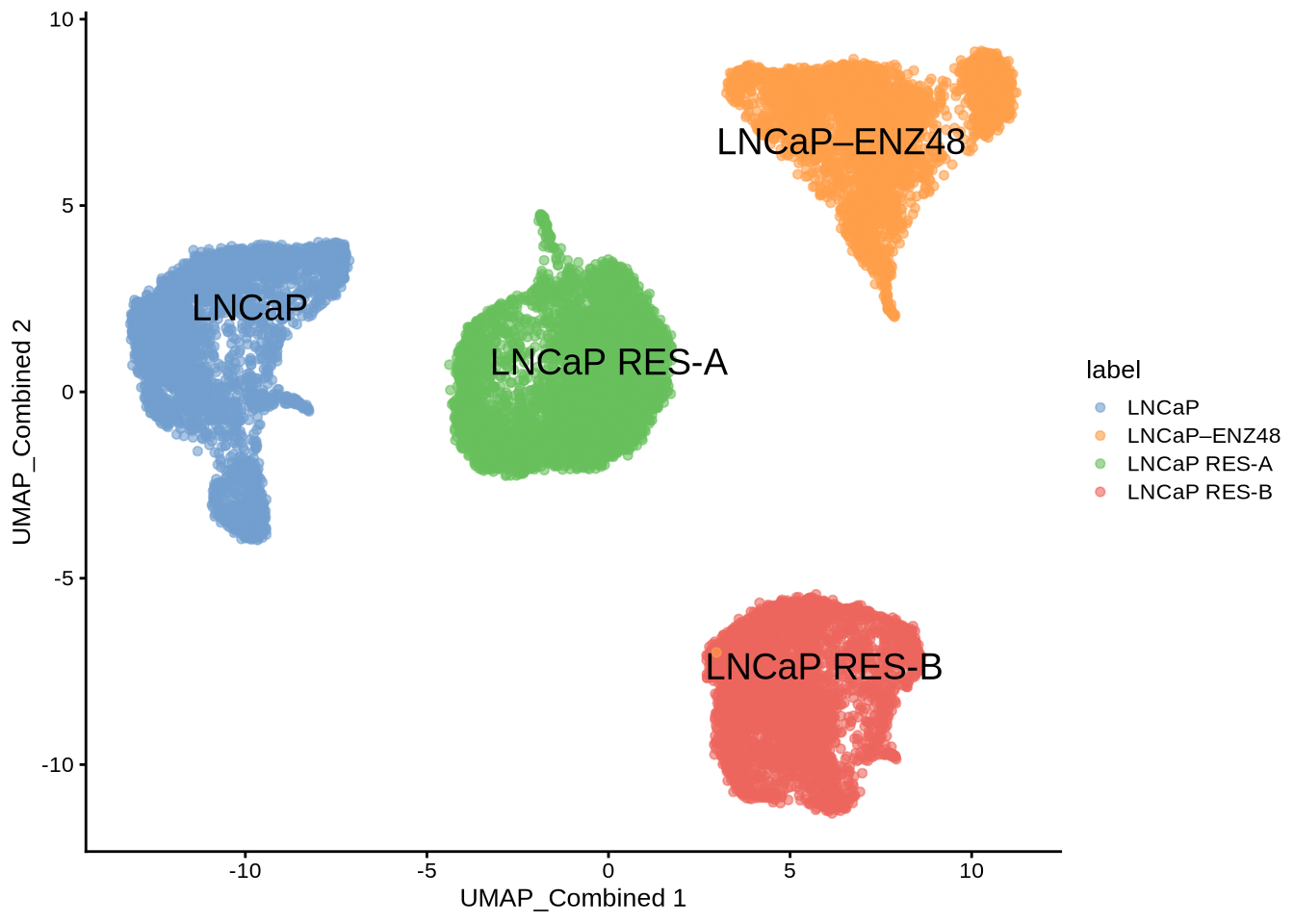
8.4 Retrieve bulk TF ChIP-seq binding sites
We retrieve TF binding sites compiled from ChIP-Atlas and ENCODE ChIP-seq. Currently, human genomes hg19 and hg38 and mouse mm10 are available.
## GRangesList object of length 1558:
## $AEBP2
## GRanges object with 2700 ranges and 0 metadata columns:
##          seqnames            ranges strand
##             <Rle>         <IRanges>  <Rle>
##      [1]     chr1        9792-10446      *
##      [2]     chr1     942105-942400      *
##      [3]     chr1     984486-984781      *
##      [4]     chr1   3068932-3069282      *
##      [5]     chr1   3069411-3069950      *
##      ...      ...               ...    ...
##   [2696]     chrY   8465261-8465730      *
##   [2697]     chrY 11721744-11722260      *
##   [2698]     chrY 11747448-11747964      *
##   [2699]     chrY 19302661-19303134      *
##   [2700]     chrY 19985662-19985982      *
##   -------
##   seqinfo: 25 sequences from an unspecified genome; no seqlengths
##
## ...
## <1557 more elements>
8.5 Link ATAC-seq peaks to target genes
We compute peak to gene correlations using the addPeak2GeneLinks function from the ArchR package. The user would need
to supply a path to an ArchR project already containing peak and gene matrices, as well as Latent semantic indexing (LSI) dimensionality reduction. We will use the joint reducedDims - “LSI_Combined”.
p2g <- calculateP2G(ArchR_path = archR_project_path,
                    useDim = "iLSI_Combined",
                    useMatrix = "GeneIntegrationMatrix",
                    threads = 1)
## Using ArchR to compute peak to gene links...## DataFrame with 17979 rows and 8 columns
## idxATAC chr start end idxRNA target Correlation distance
## <integer> <factor> <integer> <integer> <integer> <character> <numeric> <numeric>
## 1 15 chr1 912762 913262 7 NOC2L 0.546722 46297
## 2 15 chr1 912762 913262 8 KLHL17 0.516539 47575
## 3 25 chr1 920261 920761 7 NOC2L 0.649425 38798
## 4 25 chr1 920261 920761 8 KLHL17 0.637711 40076
## 5 32 chr1 927728 928228 7 NOC2L 0.610240 31331
## ... ... ... ... ... ... ... ... ...
## 17975 210643 chrX 154542721 154543221 23496 CH17-340M24.3 0.611273 114492
## 17976 210643 chrX 154542721 154543221 23501 LAGE3 0.698033 63714
## 17977 210643 chrX 154542721 154543221 23506 IKBKG 0.518586 1716
## 17978 210643 chrX 154542721 154543221 23509 DKC1 0.526624 219771
## 17979 210665 chrX 154815200 154815700 23515 F8 0.547783 2114908.6 Add TF occupancy data to peaks
The next step is to add the TF binding information by overlapping the regions of the peak matrix with the bulk ChIP-seq data. Users can supply an ArchR project path and this function will retrieve the positions of the peaks from the peak matrix.
8.7 Generate regulons
A long format data frame, representing the inferred regulons, is then generated. Three columns are important:
- transcription factors (tf)
- target genes (target)
- peak to gene correlation between tf and target gene (corr)
## DataFrame with 2776926 rows and 10 columns
##           idxATAC      chr     start       end    idxRNA      target      corr  distance     idxTF          tf
##         <integer> <factor> <integer> <integer> <integer> <character> <numeric> <numeric> <integer> <character>
## 1              15     chr1    912762    913262         7       NOC2L  0.546722     46297         4        AGO1
## 2              15     chr1    912762    913262         7       NOC2L  0.546722     46297        11      ARID4B
## 3              15     chr1    912762    913262         7       NOC2L  0.546722     46297        12      ARID5B
## 4              15     chr1    912762    913262         7       NOC2L  0.546722     46297        30        BCOR
## 5              15     chr1    912762    913262         7       NOC2L  0.546722     46297        36        BRD4
## ...           ...      ...       ...       ...       ...         ...       ...       ...       ...         ...
## 2776922    210665     chrX 154815200 154815700     23515          F8  0.547783    211490      1146       NFRKB
## 2776923    210665     chrX 154815200 154815700     23515          F8  0.547783    211490      1175      POLR2H
## 2776924    210665     chrX 154815200 154815700     23515          F8  0.547783    211490      1273      ZBTB8A
## 2776925    210665     chrX 154815200 154815700     23515          F8  0.547783    211490      1456      ZNF589
## 2776926    210665     chrX 154815200 154815700     23515          F8  0.547783    211490      1457      ZNF592
8.8 (Optional) Annotate with TF motifs
In this example, we will filter the regulons for the presence of transcription factor motifs and continue the workflow with the regulon.motif object. However, if users prefer to retain all target genes, they may proceed with the regulon object.
8.10 Add Weights
Before we calculate AR activity, we visualize its expression and show that enzalutamide does not decrease AR expression despite being an AR antagonist.
library(epiregulon.extra)
plotActivityDim(sce = GeneExpressionMatrix,
                activity_matrix = assay(GeneExpressionMatrix),
                tf = "AR",
                dimtype = "UMAP_Combined",
                label = "label",
                point_size = 1,
                legend.label = "gene expression")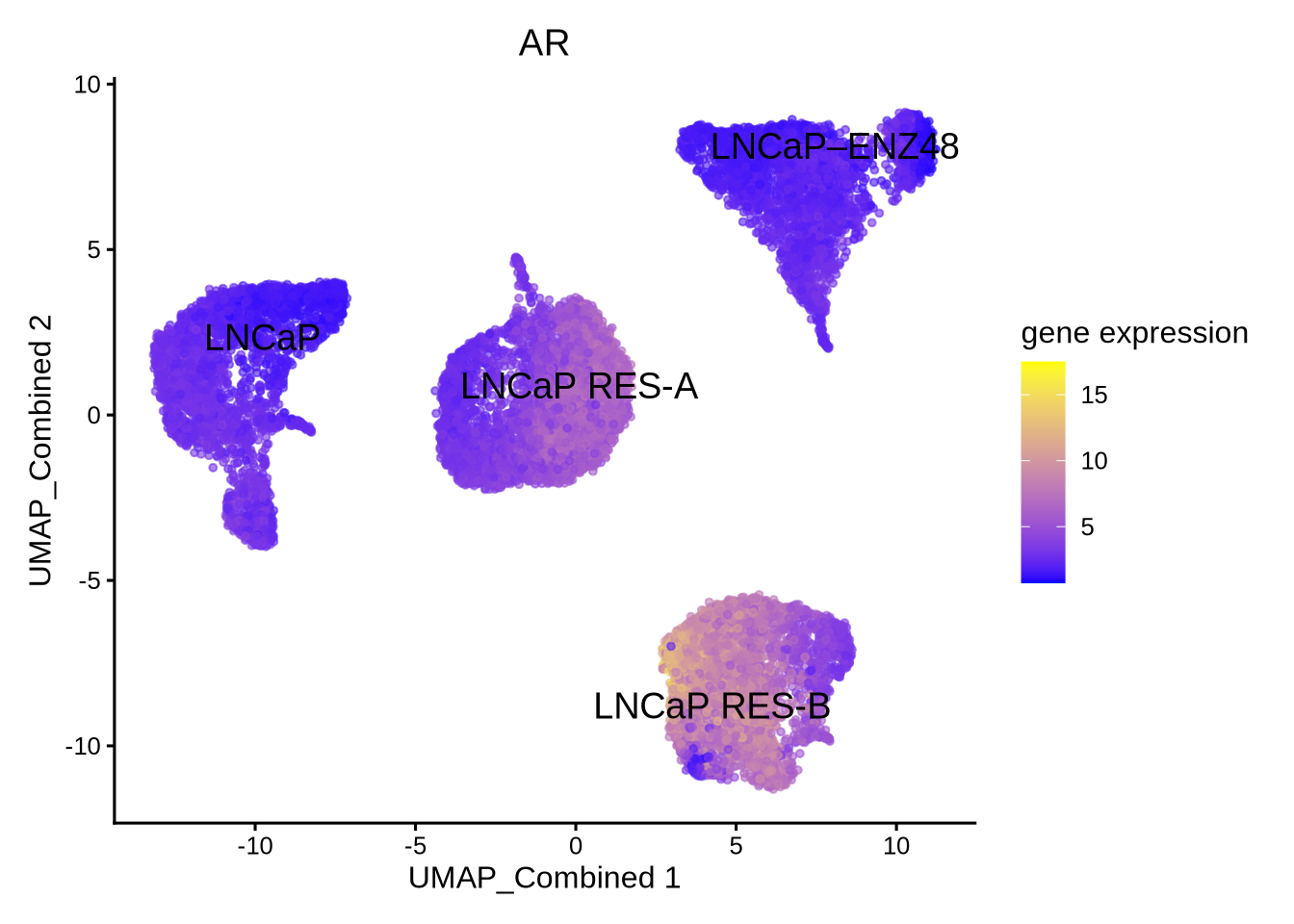
Then we extract the chromVarMatrix from ArchR project and visualize the chromatin accessibility at AR bound sites. We can see that 48 hour of enzalutamide treatment reduced chromatin accessibility at AR bound sites.
chromVarMatrix <- getMatrixFromProject(
    ArchRProj = proj,
    useMatrix = "MotifMatrix",
    useSeqnames = NULL,
    verbose = TRUE,
    binarize = FALSE,
    threads = 1
)

plotActivityDim(sce = GeneExpressionMatrix,
                activity_matrix = assay(chromVarMatrix, "z"),
                tf = "AR_689",
                dimtype = "UMAP_Combined",
                label = "label",
                point_size = 1,
                legend.label = "chromVar")
Next, we are going to compare 3 different weight methods. In the first method, the wilcoxon test compares target gene expression in cells meeting both the TF expression and accessibility cutoffs vs cells failing either the TF expression or/and accessibility cutoffs. Next, we try out the correlation method which comes in two flavors. When tf_re.merge = FALSE, weight is computed on the correlation of target gene expression vs TF gene expression. When tf_re.merge = TRUE, weight is computed on the correlation of target gene expression vs the product of TF expression and chromatin accessibility at TF-bound regulatory elements.
regulon.w.wilcox <- addWeights(regulon = pruned.regulon,
                        expMatrix = GeneExpressionMatrix,
                        exp_assay = "normalizedCounts",
                        peakMatrix = PeakMatrix,
                        peak_assay = "counts",
                        clusters = GeneExpressionMatrix$label,
                        method = "wilcoxon")

regulon.w.corr <- addWeights(regulon = pruned.regulon,
                        expMatrix = GeneExpressionMatrix,
                        exp_assay = "normalizedCounts",
                        peakMatrix = PeakMatrix,
                        peak_assay = "counts",
                        clusters = GeneExpressionMatrix$label,
                        method = "corr")

regulon.w.corr.re <- addWeights(regulon = pruned.regulon,
                        expMatrix = GeneExpressionMatrix,
                        exp_assay = "normalizedCounts",
                        peakMatrix = PeakMatrix,
                        peak_assay = "counts",
                        clusters = GeneExpressionMatrix$label,
                        method = "corr",
                        tf_re.merge = TRUE)
8.11 Calculate TF activity
Finally, the activities for a specific TF in each cell are computed by averaging the weighted expressions of target genes linked to the TF. \[y=\frac{1}{n}\sum_{i=1}^{n} x_i * weight_i\] where \(y\) is the activity of a TF for a cell \(n\) is the total number of targets for a TF \(x_i\) is the log count expression of target i where i in {1,2,…,n} \(weight_i\) is the weight of TF and target i
We calculate the activities corresponding to three weight methods.
score.combine.wilcox <- calculateActivity(expMatrix = GeneExpressionMatrix,
                                   exp_assay = "normalizedCounts",
                                   regulon = regulon.w.wilcox,
                                   normalize = TRUE,
                                   mode = "weight")
score.combine.corr <- calculateActivity(expMatrix = GeneExpressionMatrix,
                                   exp_assay = "normalizedCounts",
                                   regulon = regulon.w.corr,
                                   normalize = TRUE,
                                   mode = "weight")
score.combine.corr.re <- calculateActivity(expMatrix = GeneExpressionMatrix,
                                   exp_assay = "normalizedCounts",
                                   regulon = regulon.w.corr.re,
                                   normalize = TRUE,
                                   mode = "weight")
We visualize the different activities side by side.
library(epiregulon.extra)
plotActivityViolin(activity_matrix = score.combine.wilcox,
                   tf = c( "AR"),
                   clusters = GeneExpressionMatrix$label) + ggtitle ("AR activity by wilcoxon")
plotActivityViolin(activity_matrix = score.combine.corr,
                   tf = c( "AR"),
                   clusters = GeneExpressionMatrix$label) + ggtitle ("AR activity by corr TF vs TG")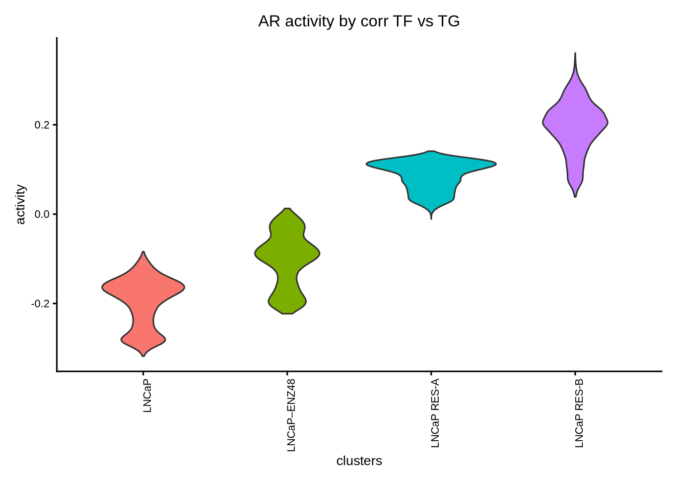
plotActivityViolin(activity_matrix = score.combine.corr.re,
                   tf = c( "AR"),
                   clusters = GeneExpressionMatrix$label) + ggtitle ("AR activity by corr TF*RE vs TG")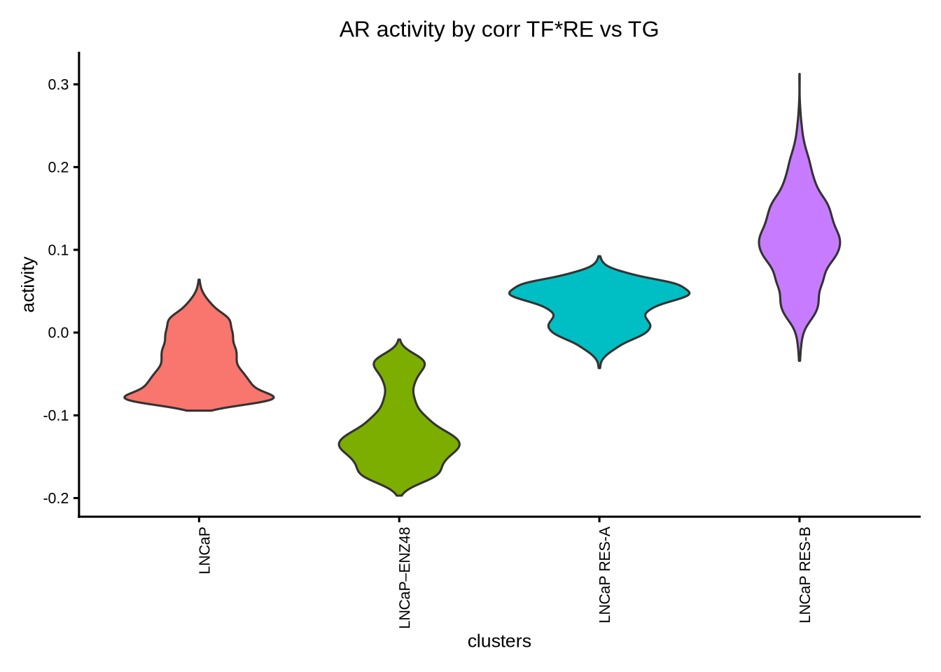
We can see that the AR activity calculated from correlation based on TF and TG expression is clearly wrong because AR activity is increased after enzalutamide treatment despite it being an AR antagonist. Therefore, for drug treatment which often decouples TF gene expression from its activity, it is important to take into consideration both TF gene expression and RE chromatin accessibility; the latter may be a better indicator of TF function. In this case, the recommended methods are either wilcox or corr with tf_re.merge = TRUE.
The astute users could however detect a difference in the prediction of the AR activity in the resistant clones “RES-A” and “RES-B” with respect to the parental “LNCaP” between the two methods. For example, the corr with tf_re.merge = TRUE shows increased AR activity in “RES-B” compared to “LNCaP” because “RES-B” shows increased AR expression. In contrast, the wilcoxon method did not predict an increase in AR activity in “RES-B” because “RES-B” still shows reduced chromatin accessibility compared to “LNCaP”. Since wilcoxon takes into account the co-occurrence of both TF gene expression and RE chromatin accessibility, this method does not predict an overall increase in AR activity.
In the absence of the ground truth, it is difficult to judge which method is superior. Therefore, it is always crucial to validate key findings with empirical evidence. The most important disclaimer we wish to make is that all predictions by epiregulon should be robustly tested experimentally.
8.12 Perform differential activity
For the remaining steps, we continue with activity derived from the wilcoxon method.
markers <- findDifferentialActivity(activity_matrix = score.combine.wilcox,
                                    clusters = GeneExpressionMatrix$label,
                                    pval.type = "some",
                                    direction = "any",
                                    test.type = "t",
                                    logvalues = FALSE  )
markers
## List of length 4
## names(4): LNCaP LNCaP–ENZ48 LNCaP RES-A LNCaP RES-BTake the top differential TFs. Summary represents comparison of cells in the indicated class vs all the remaining cells.
##    p.value FDR summary.diff       class    tf
## 1        0   0   0.06918392       LNCaP  HES4
## 3        0   0   0.05180702       LNCaP SPDEF
## 11       0   0   0.05553992 LNCaP–ENZ48  HES4
## 31       0   0  -0.03564181 LNCaP–ENZ48 NR2F6
## 12       0   0   0.07761191 LNCaP RES-A  ATF5
## 2        0   0  -0.03724509 LNCaP RES-A   EHF
## 21       0   0   0.04959529 LNCaP RES-B   JUN
## 32       0   0   0.04786785 LNCaP RES-B NR2F2
8.13 Visualize the results
First visualize the known differential TFs by bubble plot
plotBubble(activity_matrix = score.combine.wilcox,
           tf = c("AR","FOXA1", "MYC","JUN"),
           pval.type = "some",
           direction = "up",
           clusters = GeneExpressionMatrix$label,
           logvalues = FALSE)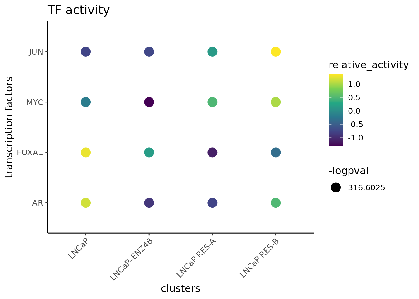
Then visualize the most differential TFs by clusters
plotBubble(activity_matrix = score.combine.wilcox,
           tf = unique(markers.sig$tf),
           pval.type = "some",
           direction = "any",
           clusters = GeneExpressionMatrix$label,
           logvalues = FALSE)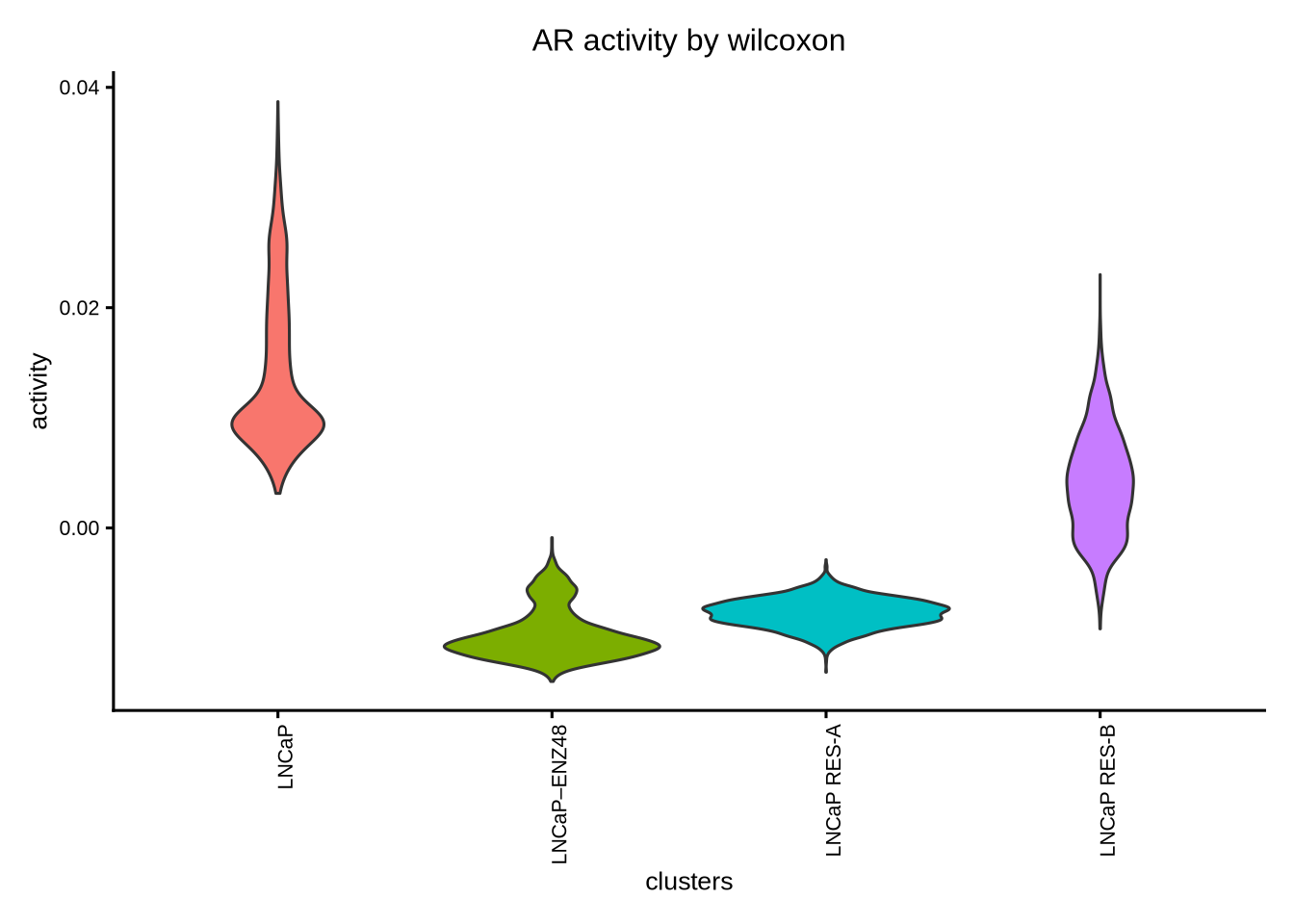
Visualize the known differential TFs by UMAP
plotActivityDim(sce = GeneExpressionMatrix,
                activity_matrix = score.combine.wilcox,
                tf = c( "AR", "FOXA1", "MYC", "JUN"),
                dimtype = "UMAP_Combined",
                label = "label",
                point_size = 1,
                ncol = 2,
                nrow = 2)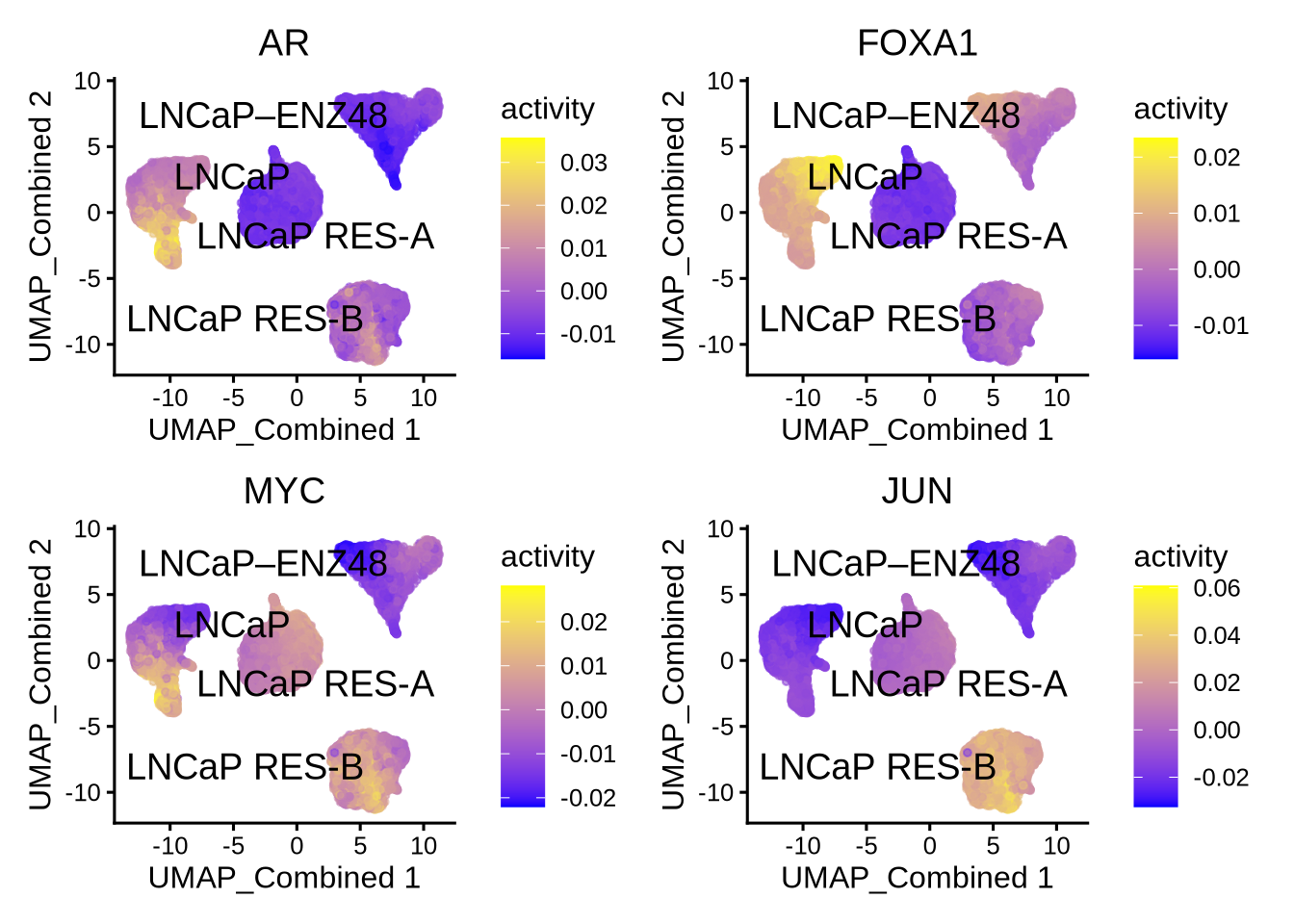
Visualize the differential TFs by UMAP
plotActivityDim(sce = GeneExpressionMatrix,
                activity_matrix = score.combine.wilcox,
                tf = markers.sig$tf[1:4],
                dimtype = "UMAP_Combined",
                label = "label",
                point_size = 1,
                ncol = 2,
                nrow = 2)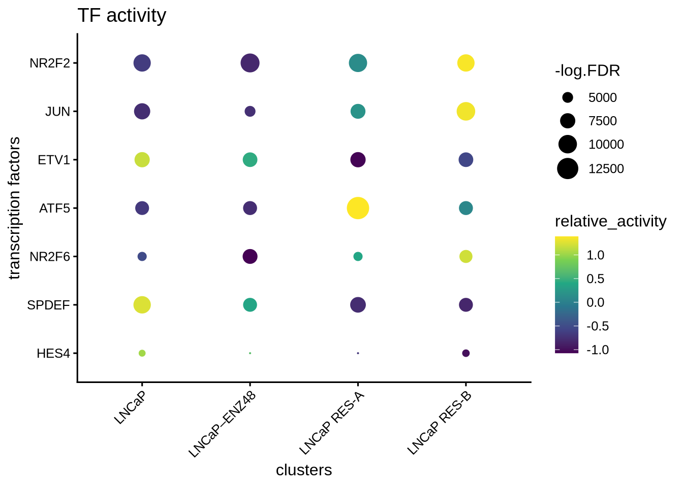
Visualize regulons by heatmap
rowData(GeneExpressionMatrix) <- NULL

plotHeatmapRegulon(sce=GeneExpressionMatrix,
                   tfs= c( "AR", "FOXA1", "MYC", "JUN"),
                   regulon=regulon.w.wilcox,
                   regulon_cutoff=0.1,
                   downsample=1000,
                   cell_attributes="label",
                   col_gap="label",
                   exprs_values="normalizedCounts",
                   name="regulon heatmap",
                   column_title_rot = 45)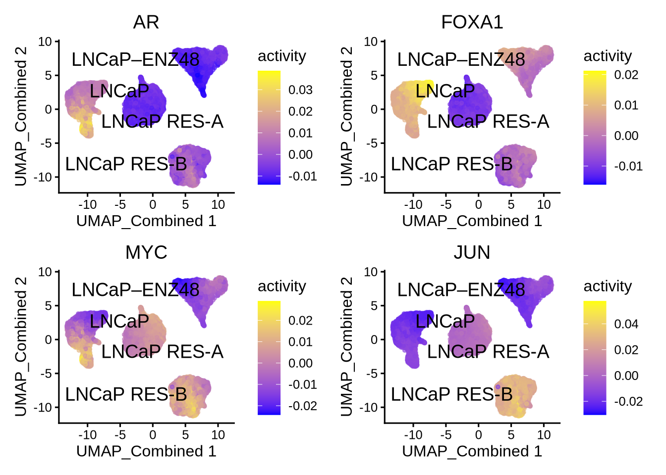
plotHeatmapActivity(activity=score.combine.wilcox,
                    sce=GeneExpressionMatrix,
                    tfs=rownames(score.combine.wilcox),
                    downsample=1000,
                    cell_attributes="label",
                    col_gap="label",
                    name = "transcription factor activity",
                    column_title_rot = 45)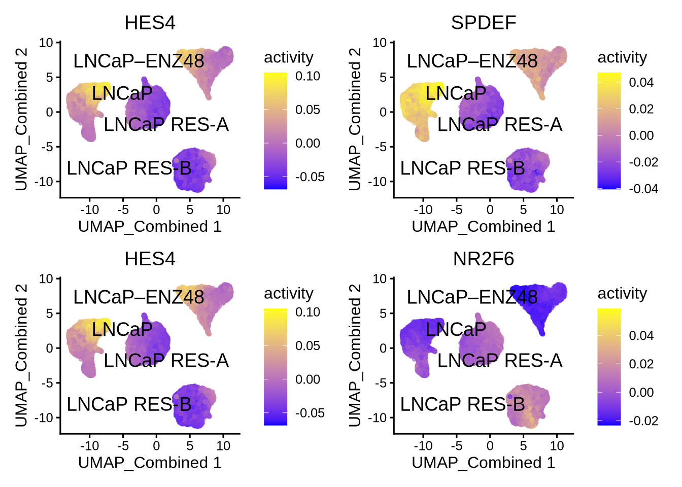
8.14 Geneset enrichment
Sometimes we are interested to know what pathways are enriched in the regulon of a particular TF. We can perform geneset enrichment using the enricher function from clusterProfiler.
#retrieve genesets
H <- EnrichmentBrowser::getGenesets(org = "hsa",
                                    db = "msigdb",
                                    cat = "H",
                                    gene.id.type = "SYMBOL",
                                    cache = FALSE)
C6 <- EnrichmentBrowser::getGenesets(org = "hsa",
                                     db = "msigdb",
                                     cat = "C6",
                                     gene.id.type = "SYMBOL",
                                     cache = FALSE)

#combine genesets and convert genesets to be compatible with enricher
gs <- c(H,C6)
gs.list <- do.call(rbind,lapply(names(gs),
                                function(x) {data.frame(gs=x, genes=gs[[x]])}))

enrichresults <- regulonEnrich(TF = c("AR", "FOXA1", "MYC", "JUN"),
                               regulon = regulon.w.wilcox,
                               weight = "weight",
                               weight_cutoff = 0,
                               genesets = gs.list)

#plot results
enrichPlot(results = enrichresults, ncol = 2)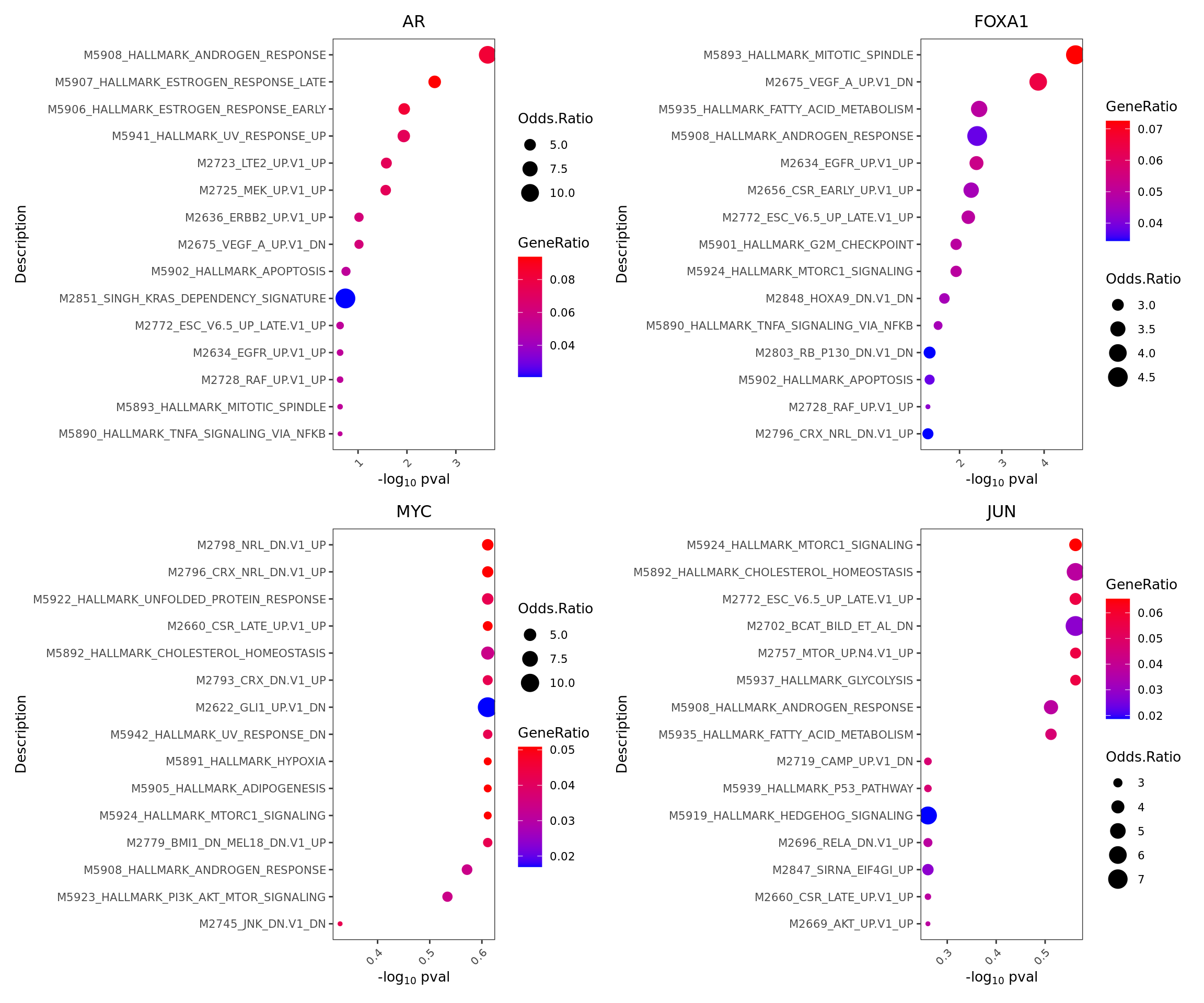
We can visualize the genesets of known factors as a network
plotGseaNetwork(tf = names(enrichresults),
                enrichresults = enrichresults,
                p.adj_cutoff = 0.1,
                ntop_pathways = 10)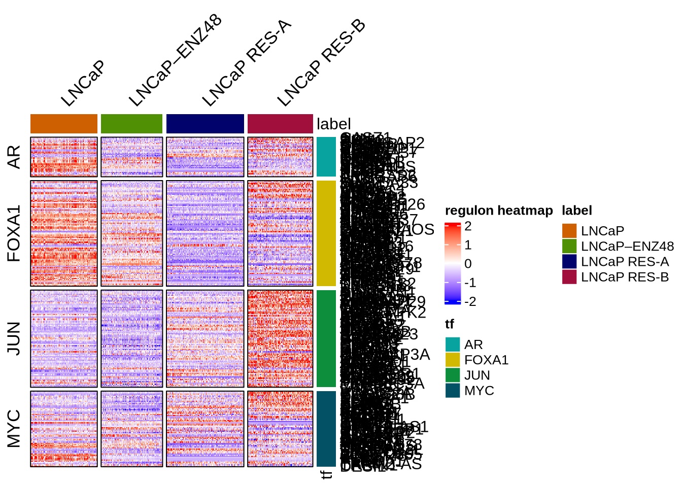
We can visualize the genesets of differential factors as a network
enrichresults <- regulonEnrich(TF = markers.sig$tf,
                               regulon = regulon.w.wilcox,
                               weight = "weight",
                               weight_cutoff = 0,
                               genesets = gs.list)
plotGseaNetwork(tf = names(enrichresults),
                enrichresults = enrichresults,
                p.adj_cutoff = 0.1,
                ntop_pathways = 10)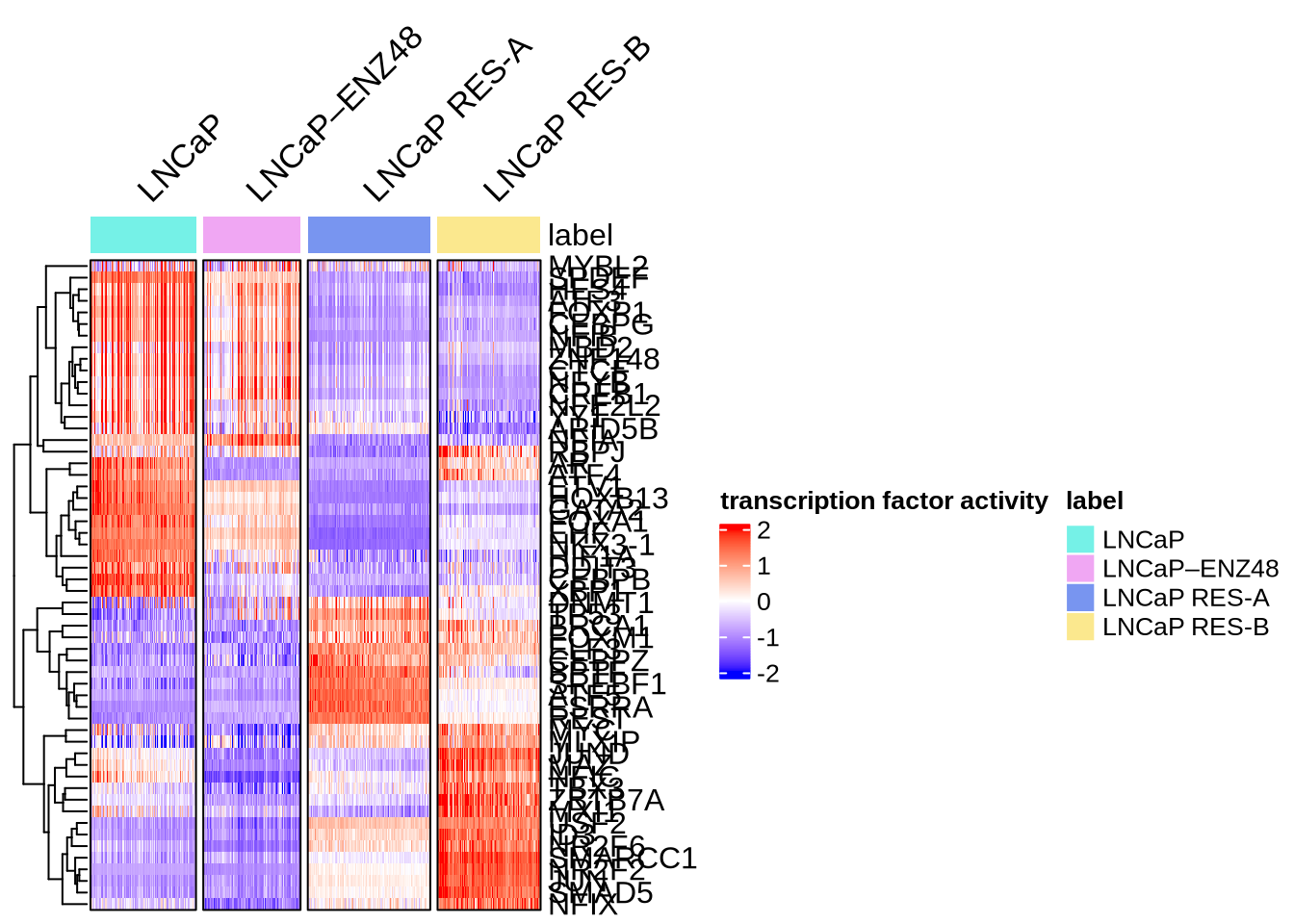
8.15 Differential network analysis {diff_network}
In addition to looking at summed TF activity, a second approach to investigate differential TF activity is to compare target genes or network topology. In this example, we know that AR is downregulated in the enzalutamide treated cells compared to parental LNCaP.
We perform edge subtracted graph between two conditions and rank TFs by degree centrality. In this example, positive centrality indicates higher activity in parental LNCaP and negative centrality indicates higher activity in enzalutamide treated cells.
# construct a graph of the parental and enzalutamide treated cells respectively
LNCaP_network <- buildGraph(regulon.w.wilcox, weights = "weight", cluster="LNCaP")
ENZ_network <- buildGraph(regulon.w.wilcox, weights = "weight", cluster="LNCaP–ENZ48")

# construct a difference graph
diff_graph <- buildDiffGraph(LNCaP_network, ENZ_network, abs_diff = FALSE)
diff_graph <- addCentrality(diff_graph)
diff_graph <- normalizeCentrality(diff_graph)
rank_table <- rankTfs(diff_graph)

library(ggplot2)
ggplot(rank_table, aes(x = rank, y = centrality)) +
    geom_point() +
    ggrepel::geom_text_repel(data = rbind(head(rank_table,5),
                                          tail(rank_table,5)),
                             aes(label = tf),
                             nudge_x = 0, nudge_y = 0, box.padding = 0.5) +
    theme_classic() + ggtitle ("differential TFs (LNCaP-ENZ) ranked by degree centrality")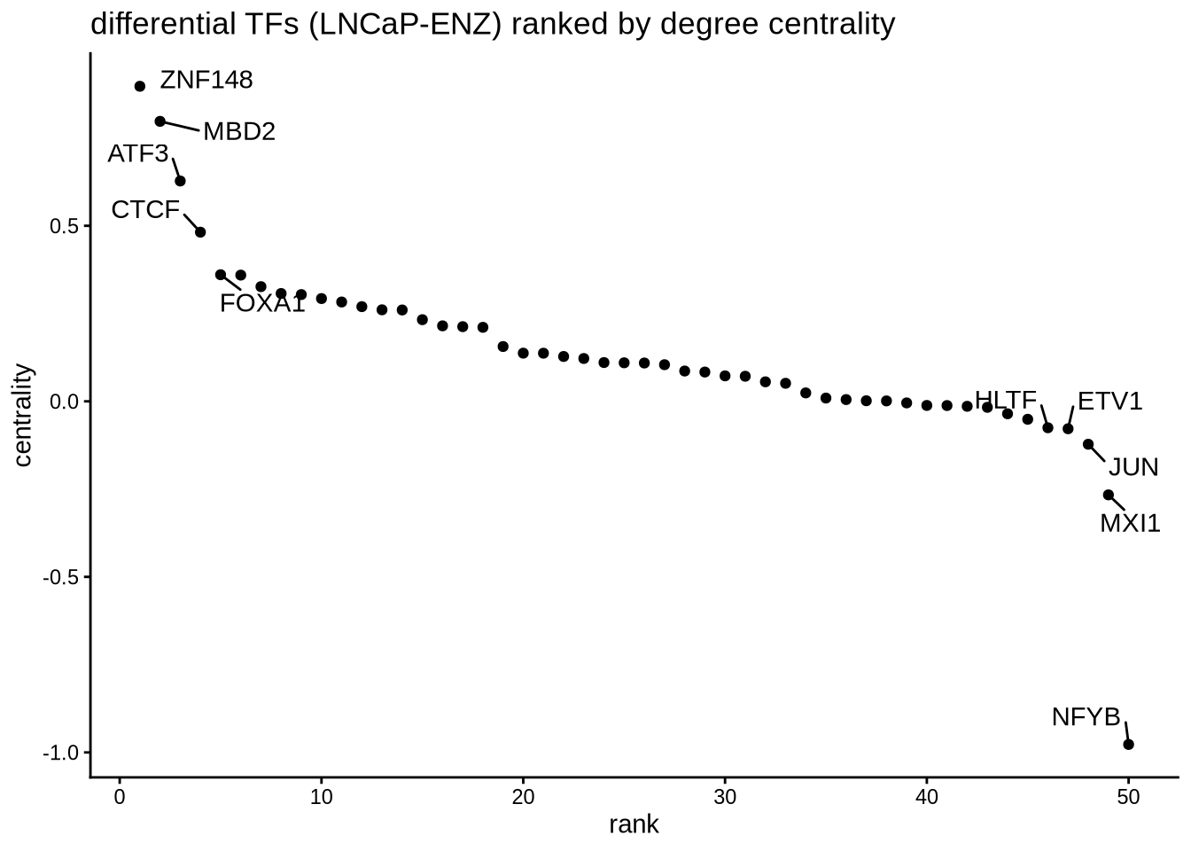
Sometimes, we are interested to identify interaction partners of the TFs of interest. This can be achieved by comparing the overlap of the targets genes for all the TFs and identify the most similar TFs by Jaccard similarity. To illustrate this function, we take a look at the top most similar 20 TFs to AR.
library(igraph)
diff_graph_filter <- subgraph.edges(diff_graph,
                                    E(diff_graph)[E(diff_graph)$weight>0],
                                    del=TRUE)


# compute a similarity matrix of all TFs
similarity_score <- calculateJaccardSimilarity(diff_graph_filter)

# Focus on AR
similarity_score_AR <- similarity_score[, "AR"]
similarity_df <- data.frame(similarity = head(sort(similarity_score_AR,
                                                   decreasing = TRUE),20),
                            TF = names(head(sort(similarity_score_AR,
                                                 decreasing = TRUE),20)))

similarity_df$TF <- factor(similarity_df$TF,
                           levels = rev(unique(similarity_df$TF)))

# plot top TFs most similar to SPI1
topTFplot <- ggplot(similarity_df, aes(x=TF, y=similarity)) +
  geom_bar(stat="identity") +
  coord_flip() +
  ggtitle("AR similarity") +
  theme_classic()

print(topTFplot)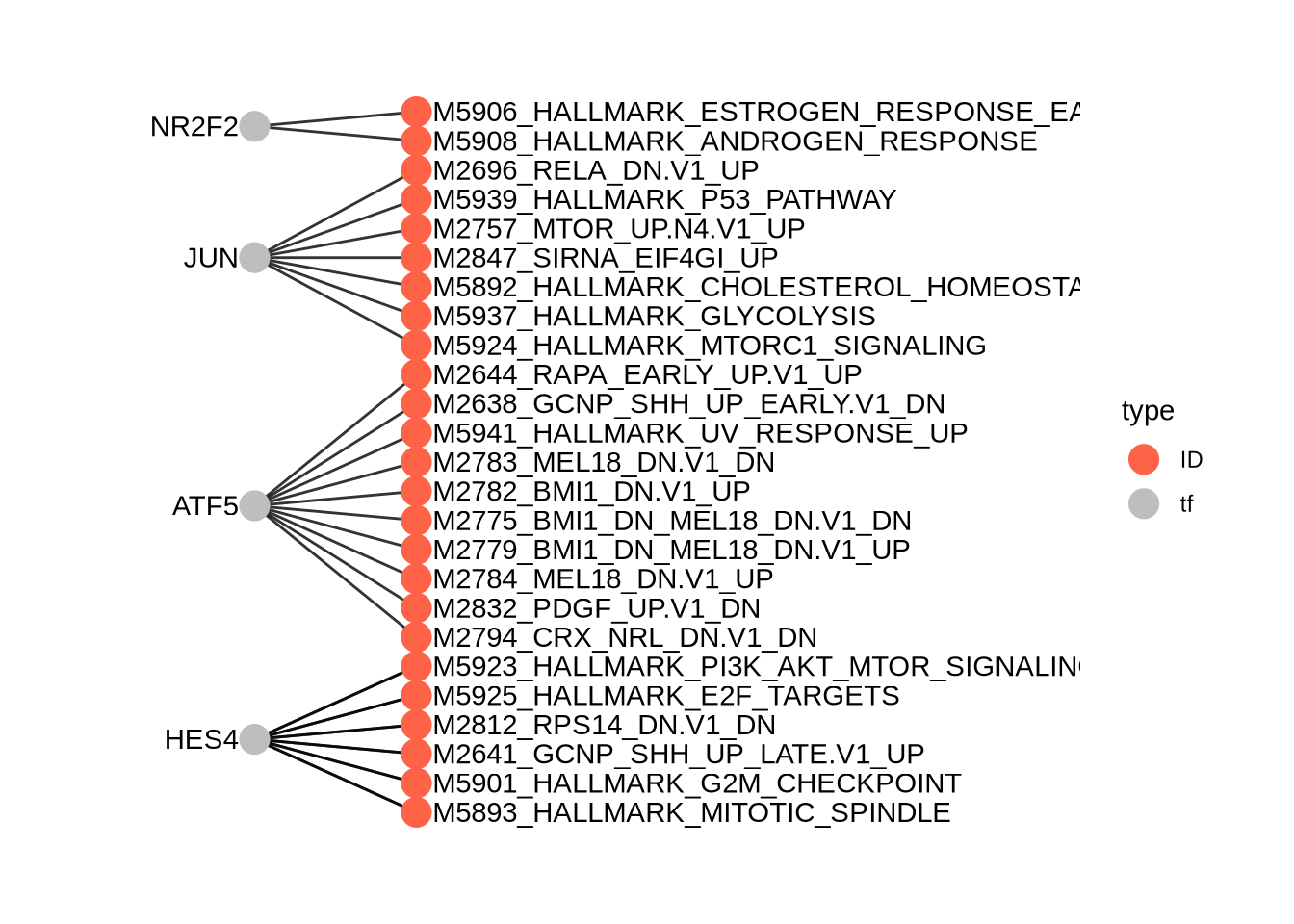
In order to convince ourselves that our differential network is statistically significant, we permute the edges and obtain a background graph from averaging many iterations. Here, we plot the differential network graph subtracted by permuted graphs.
# create a permuted graph by rewiring the edges 100 times
permute_matrix <- permuteGraph(diff_graph_filter, "AR", 100, p=1)
permute_matrix <- permute_matrix[names(similarity_score_AR),]
diff_matrix <- similarity_score_AR-rowMeans(permute_matrix)

diff_matrix_df <- data.frame(similarity = head(sort(diff_matrix,
                                                    decreasing = TRUE),20),
                            TF = names(head(sort(diff_matrix,
                                                 decreasing = TRUE),20)))

diff_matrix_df$TF <- factor(diff_matrix_df$TF, levels = rev(unique(diff_matrix_df$TF)))

# plot top TFs most similar to AR
topTFplot <- ggplot(diff_matrix_df, aes(x=TF, y=similarity)) +
            geom_bar(stat="identity") +
            coord_flip() +
            ggtitle("background subtracted AR similarity ") +
            theme_classic()
print(topTFplot)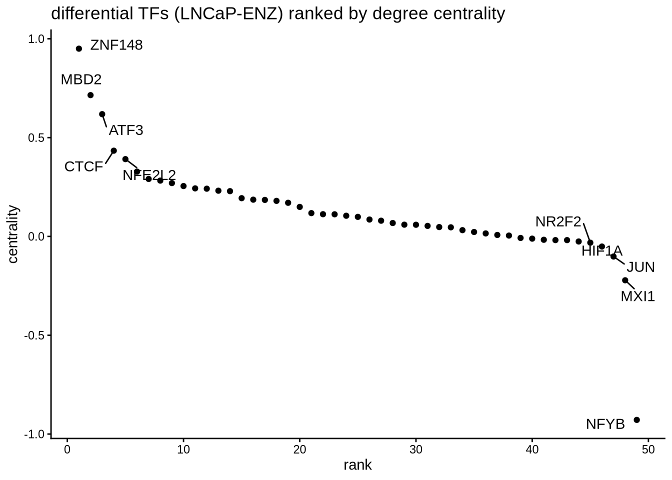
# obtain empirical p-values
p_matrix <- rowMeans(apply(permute_matrix, 2, function(x) {x > similarity_score_AR}))
p_matrix[names(head(sort(diff_matrix,decreasing = TRUE),20))]
## JUND MYC HOXB13 FOXA1 NFIC CEBPB XBP1 MAZ ATF4 CTCF REST GATA2 ETV1 FOXP1 CEBPG JUN YY1 NFIB
## 0.00 0.00 0.00 0.01 0.03 0.01 0.00 0.03 0.01 0.00 0.01 0.01 0.03 0.01 0.01 0.03 0.00 0.00
## ZNF148 USF2
## 0.00 0.01