9 Single modality: scRNA-seq only

Epiregulon also supports transcription factor activity inference when users only have scRNA-seq. To enable TF activity inference on scRNA-seq, users can supply a pre-constructed gene regulatory network. In this vignette, we bypass the regulon construction step and go straight to calculate TF activity from a Dorothea GRN.

9.1 Load regulons

Dorothea provides both human and mouse pre-constructed gene regulatory networks based on curated experimental and computational data.

library(dorothea)
data(dorothea_mm, package = "dorothea")
regulon <- dorothea_mm 

#known tfs
genes_to_plot <- c("Onecut1", "Hnf1a","Pdx1","Arx")

9.2 Load scRNA-seq data

We download the raw counts of a mouse pancreas data set from scRNAseq. We add normalized logcounts, perform dimension reduction and visualize the embeddings using scater.

library(scRNAseq)
library(scater)

sce <- BaronPancreasData('mouse')
sce <- logNormCounts(sce)
sce <- runPCA(sce)
sce <- runUMAP(sce)

plotUMAP(sce, colour_by = "label", text_by = "label")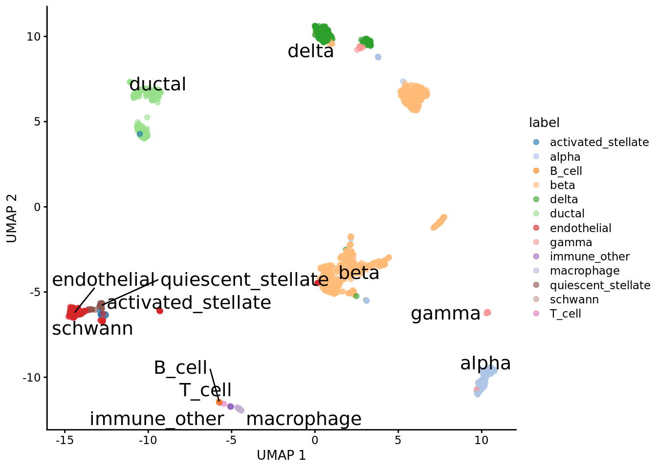

9.3 Calculate activity

Even though Dorothea provides weights under the mor column, we can achieve superior performance if we recompute the weights based on the correlation between tf and target gene expression based on our own data. We performed 2 steps: the first step is to add weights to the Dorothea regulons and the second step is to estimate the TF activity by taking the weighted average of the target gene expression.

library(epiregulon)


#Add weights to regulon. Default method (wilcoxon) cannot be used
regulon.ms <- addWeights(regulon = regulon,
                         expMatrix = sce,
                         clusters = sce$label,
                         BPPARAM = BiocParallel::MulticoreParam(),
                         method="corr")

#Calculate activity
score.combine <- calculateActivity(sce, 
                                   regulon = regulon.ms, 
                                   mode = "weight", 
                                   method = "weightedMean")

9.4 Perform differential activity

library(epiregulon.extra)
markers <- findDifferentialActivity(activity_matrix = score.combine, 
                                    clusters = sce$label, 
                                    pval.type = "some", 
                                    direction = "up", 
                                    test.type = "t")

Take the top TFs

markers.sig <- getSigGenes(markers, topgenes = 5 )

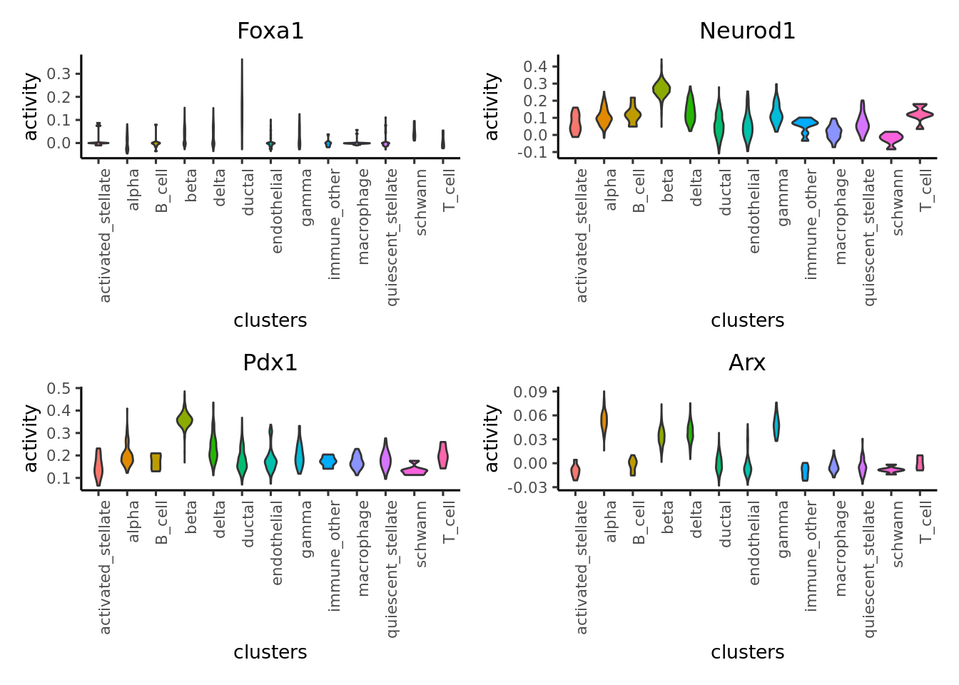
9.5 Visualize activity

Finally we visualize the TF activity by either UMAP, violin plots or bubble plots. We confirm the activity of known lineage factors: Pdx1 in beta cells, Arx in alpha cells, Onecut1 in ductal cells and Hnf1a in both endocrine and exocrine cells.

# plot umap
plotActivityDim(sce = sce, 
                activity_matrix = score.combine,
                tf = genes_to_plot, 
                legend.label = "score",
                point_size = 0.1,
                dimtype = "UMAP", 
                label = "label", 
                combine = TRUE,
                text_size = 2)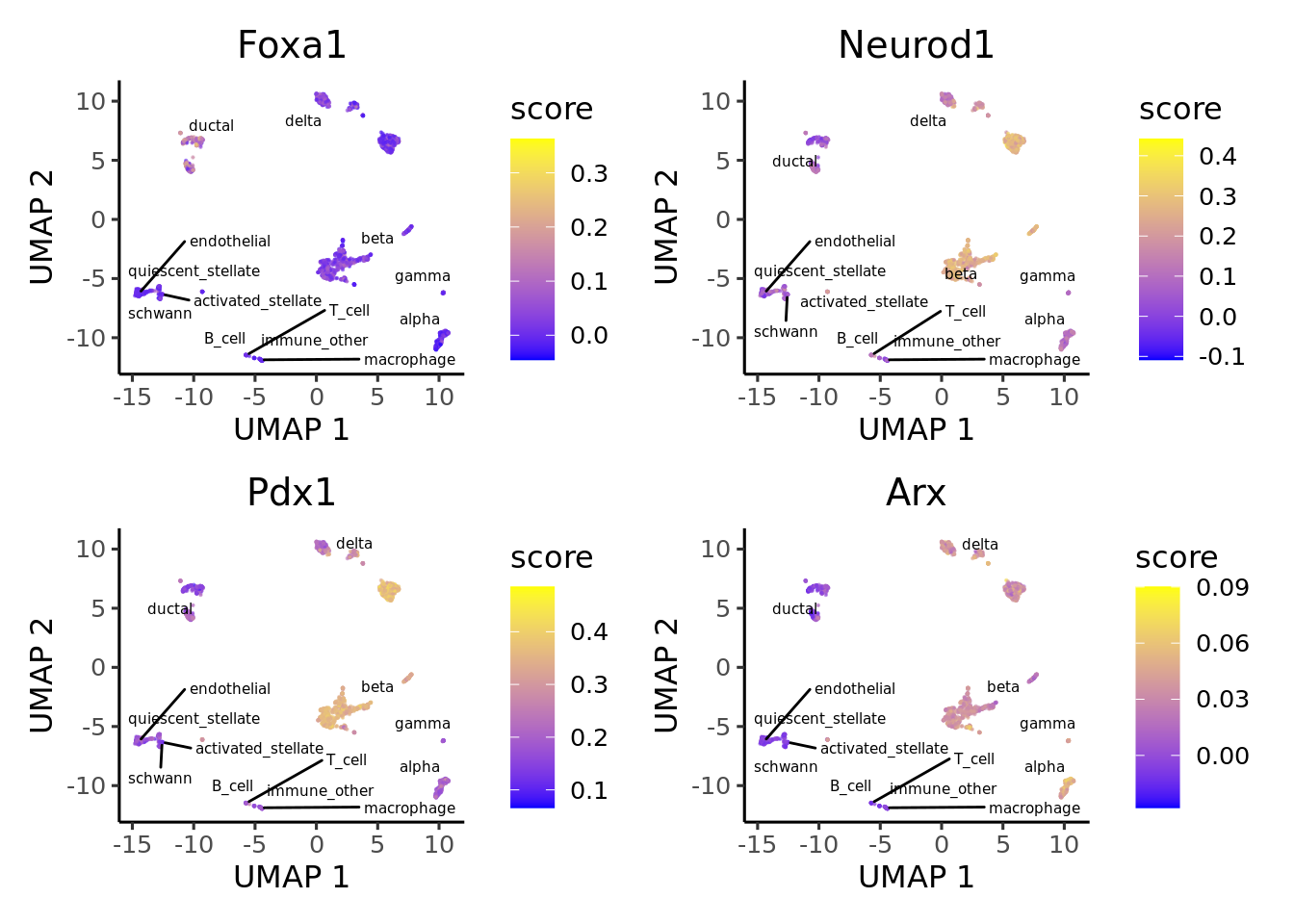

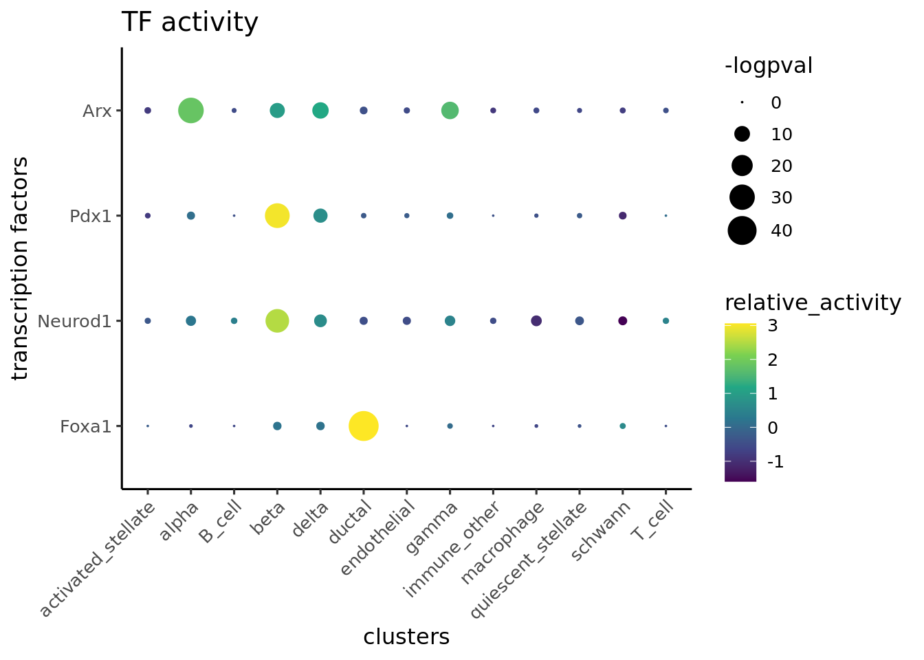
# plot violin plot
plotActivityViolin(score.combine, 
                   tf = genes_to_plot,
                   clusters = sce$label)

# plot bubble plot
plotBubble(score.combine, 
           tf = genes_to_plot, 
           clusters = sce$label)

Plot bubble plot of differential TFs

plotBubble(score.combine, 
           tf = markers.sig$tf, 
           clusters = sce$label)

We can adapt the epiregulon package to plot gene expression. When compared against TF activity, gene expression tends to have noisy signals and high dropout rates. Epiregulon enhances the signal to noise ratio of TF activity and better resolves lineage differences.

# plot umap
plotActivityDim(sce = sce, 
                activity_matrix = logcounts(sce),
                tf = genes_to_plot, 
                legend.label = "gex",
                point_size = 0.1,
                dimtype = "UMAP", 
                label = "label", 
                combine = TRUE,
                text_size = 2,
                colors = c("gray","blue"),
                limit = c(0,2))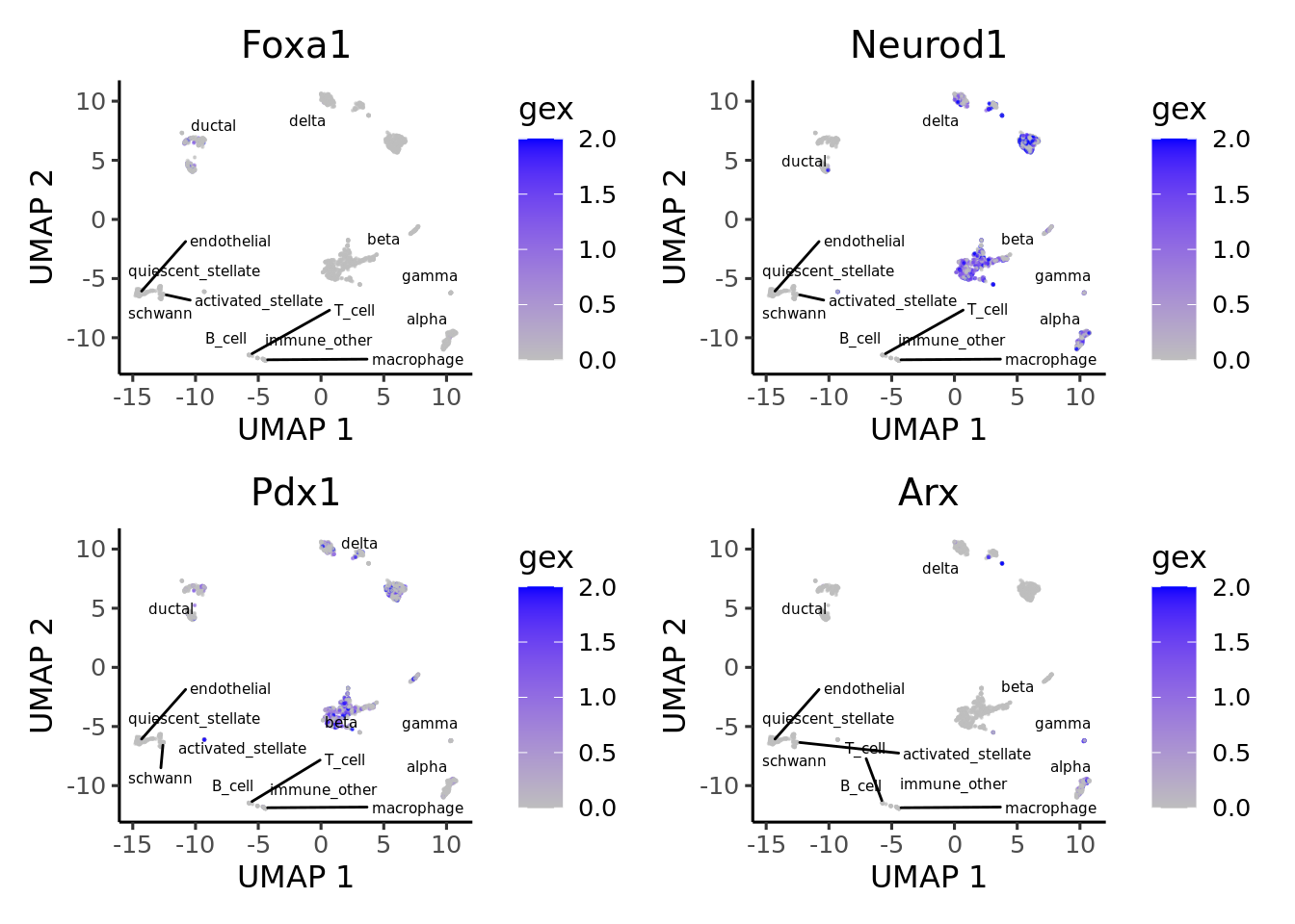

# plot violin plot
plotActivityViolin(logcounts(sce), 
                   tf = genes_to_plot,
                   clusters = sce$label,
                   legend.label = "gex")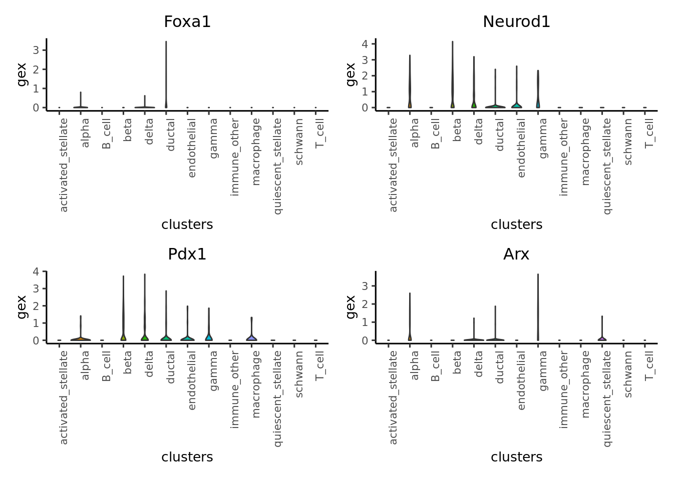

# plot Bubble plot
plotBubble(logcounts(sce), 
           tf = markers.sig$tf, 
           clusters = sce$label,
           legend.label = "gex",
           title = "gene expression")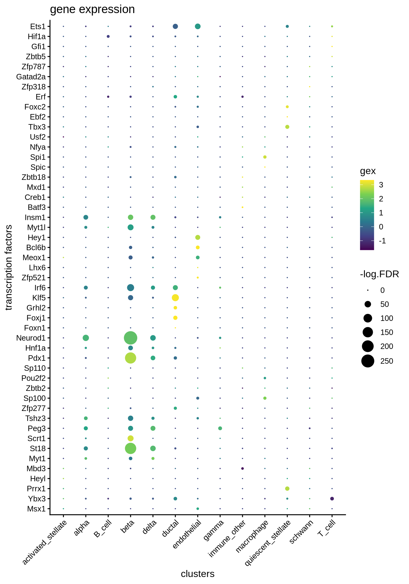

We can visualize the target genes for transcription factors of interest

plotHeatmapRegulon(sce=sce,
                   tfs=genes_to_plot,
                   regulon=regulon.ms,
                   regulon_cutoff=0.5,
                   downsample=1000,
                   cell_attributes="label",
                   col_gap="label",
                   exprs_values="logcounts",
                   name="regulon heatmap",
                   column_title_rot = 45)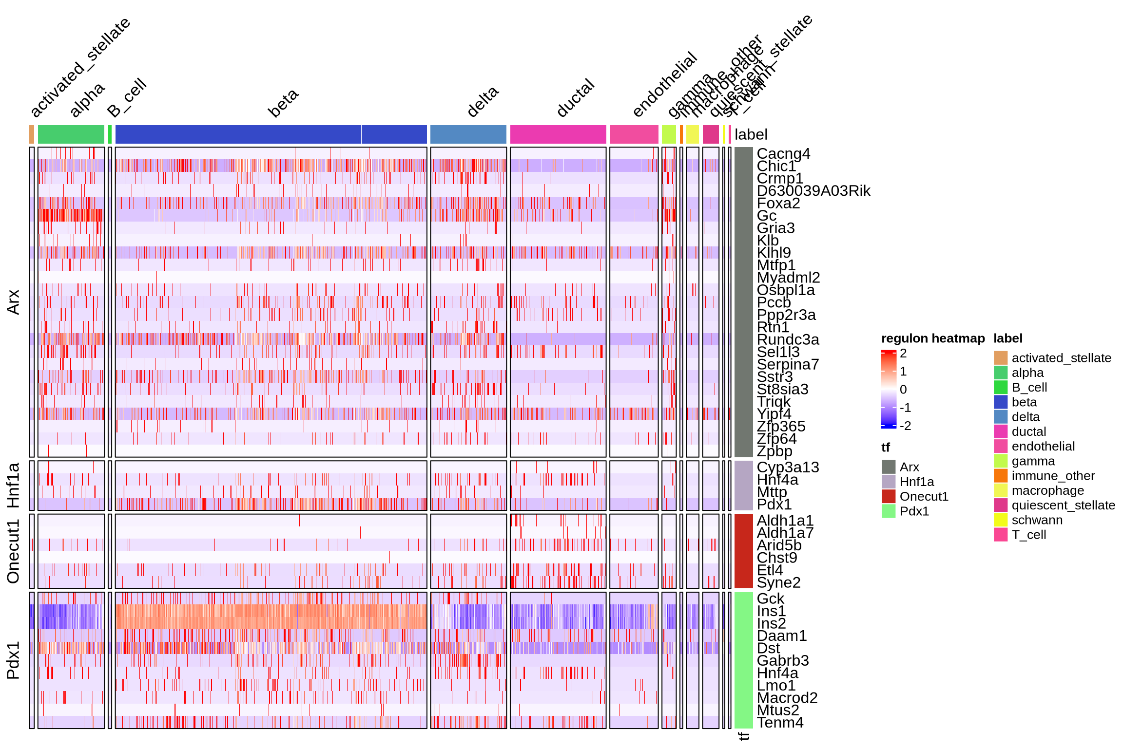

plotHeatmapActivity(activity_matrix = score.combine,
                    sce=sce,
                    tfs=genes_to_plot,
                    downsample=1000,
                    cell_attributes="label",
                    col_gap="label",
                    name="regulon heatmap",
                    column_title_rot = 45)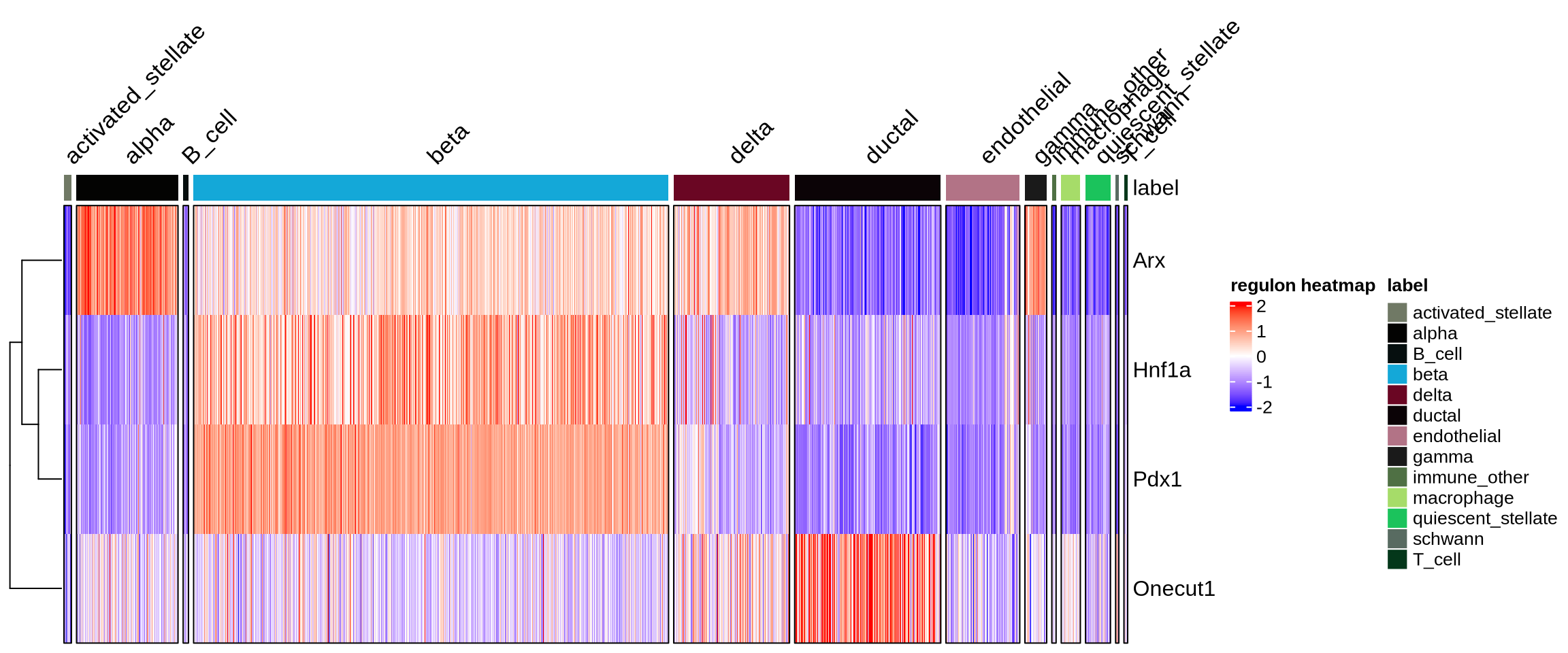

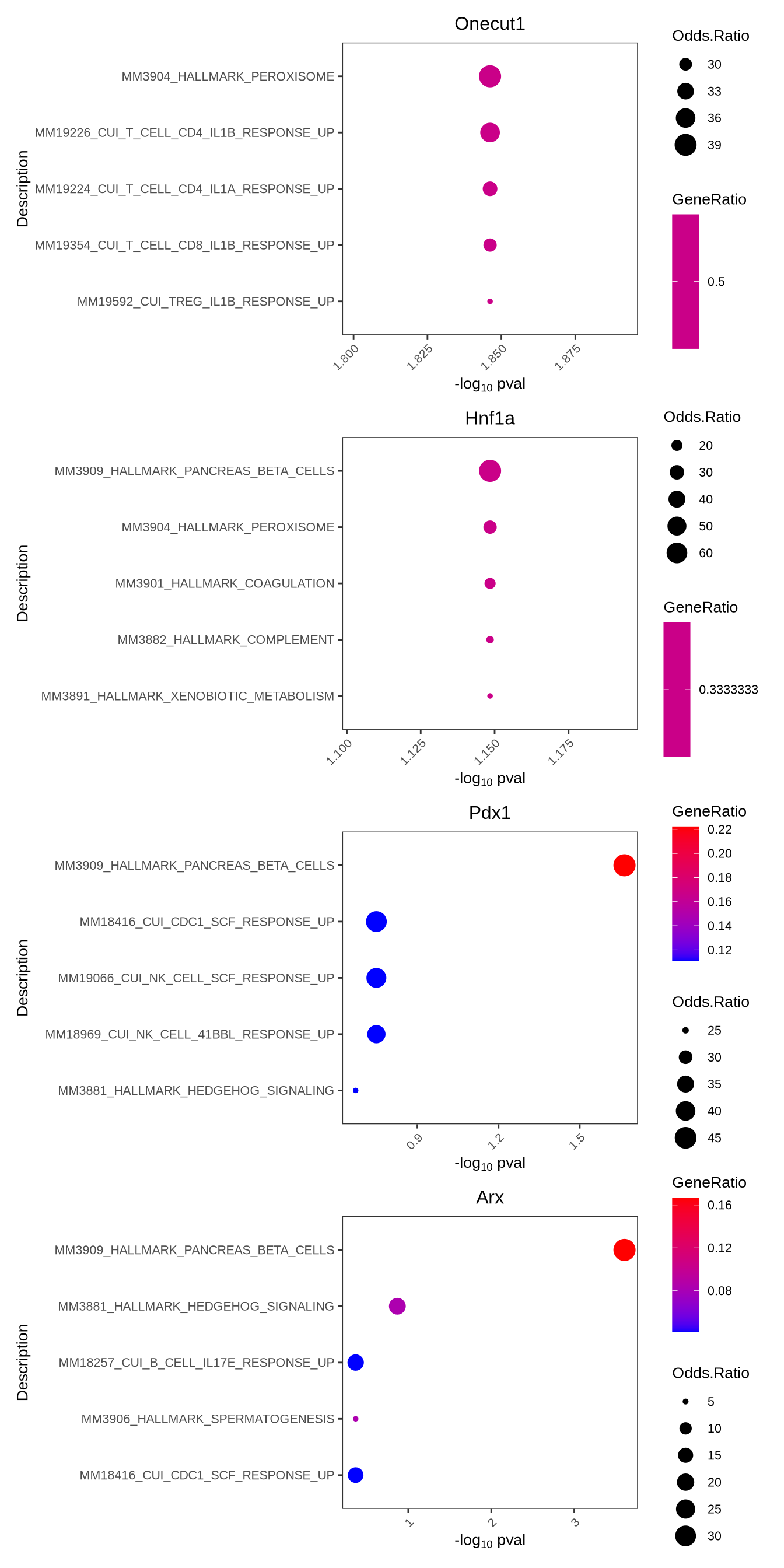
9.6 Perform pathway enrichment

Sometimes it is useful to understand what pathways are enriched in the regulons. We take the highly correlated target genes of a regulon and perform geneset enrichment using the enricher function from clusterProfiler.

#retrieve genesets
MH <- EnrichmentBrowser::getGenesets(org = "mmu", 
                                    db = "msigdb", 
                                    cat = "MH", 
                                    gene.id.type = "SYMBOL", 
                                    cache = FALSE)
M7 <- EnrichmentBrowser::getGenesets(org = "mmu", 
                                     db = "msigdb", 
                                     cat = "M7", 
                                     gene.id.type = "SYMBOL",  
                                     cache = FALSE)

#combine genesets and convert genesets to be compatible with enricher
gs <- c(MH,M7)
gs.list <- do.call(rbind,lapply(names(gs), function(x) 
  {data.frame(gs = x, genes = gs[[x]])}))

enrichresults <- regulonEnrich(genes_to_plot, 
                               regulon = regulon.ms, 
                               weight = "weight",
                               weight_cutoff = 0.3, 
                               genesets = gs.list)

#plot results
enrichPlot(results = enrichresults, ncol = 1, top=5)